9 Predicting Peel Adhesion with Machine Learning: From Rheology to N/25 mm

A good doctor does not wait for symptoms. A small blood sample and a handful of lab values – blood sugar, cholesterol, iron – already tell a lot about how healthy you are and what might go wrong in the future. Nobody has to fall ill first.

Adhesive development could work the same way. The number a tape user cares about is the peel force: how many newtons it takes to pull a 25 mm wide strip off a surface. Measuring it means making the adhesive, coating it on a backing, laminating, waiting, cutting strips and pulling them off a steel plate – often days of work per recipe. A rheometer, on the other hand, delivers the adhesive’s “lab values” in an afternoon. In this final part of the series, we ask: can those lab values predict the peel force – and even the way a tape fails – before a single peel test is run?

We will see which rheological numbers carry the information, how a machine-learning model learns from them, and – just as important – how to check honestly whether it has learned anything at all.

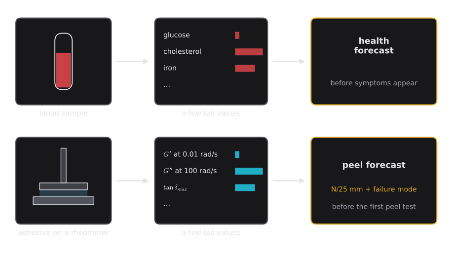
What to look for: in both rows, a small sample and a few well-chosen numbers replace a long wait. The art lies in choosing the right numbers.

The Peel Test: What We Want to Predict

In a peel test, a strip of tape of width $b$ (usually 25 mm) is bonded to a steel plate, left to rest for a defined time (for example 20 minutes or 24 hours) and then pulled off at a constant speed – typically 300 mm/min – while the force $F$ is recorded. Common standards are FINAT FTM 1, PSTC-101 and ASTM D3330. The two usual geometries differ in the angle $\theta$ between the tape and the plate: 180° (the tape is folded back on itself) and 90° (it is pulled straight up).

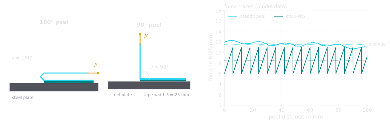
What to look for: a good tape peels with a nearly constant force. A saw-tooth trace means the tape alternately sticks and suddenly lets go – “stick-slip”.

The result is given as force per width, in N/25 mm. Behind this number lies an energy: the work needed to separate one square meter of bond, the peel energy $\mathcal{G}_a$:

$\mathcal{G}_a = \frac{F}{b}\,(1 - \cos\theta) \quad\Rightarrow\quad 180°:\ \mathcal{G}_a = \frac{2F}{b}, \qquad 90°:\ \mathcal{G}_a = \frac{F}{b}$

In words: at 180°, the pulling hand has to travel twice the peeled length (the tape folds back), so the same force does twice the work compared with 90°.

Worked example. A tape peels at 10 N/25 mm in a 180° test: $\mathcal{G}_a = 2 \times 10\ \mathrm{N} / 0.025\ \mathrm{m} = 800\ \mathrm{J/m^2}$. The energy of the chemical and physical bonds across the interface – the “true” adhesion – is only about 0.05–0.1 J/m². The peel energy is roughly ten thousand times larger. Where does the rest go? Into stretching, flowing and heating the adhesive: viscoelastic dissipation.

Why Peel Depends on Speed – and Temperature

This leads to one of the most important relations in adhesion science, found by Gent and Schultz in 1972:

$\mathcal{G}_a = \mathcal{G}_0\left[1 + \Phi(a_T\,v)\right]$

In words: the peel energy is the small “true” interfacial adhesion $\mathcal{G}_0$, multiplied by a large dissipation factor $\Phi$. This factor depends on the peel speed $v$ and on the temperature – through the same shift factor $a_T$ we met in Part 8. In other words, peel behaves like the loss modulus $G''$: faster is like colder, and more dissipation means more force.

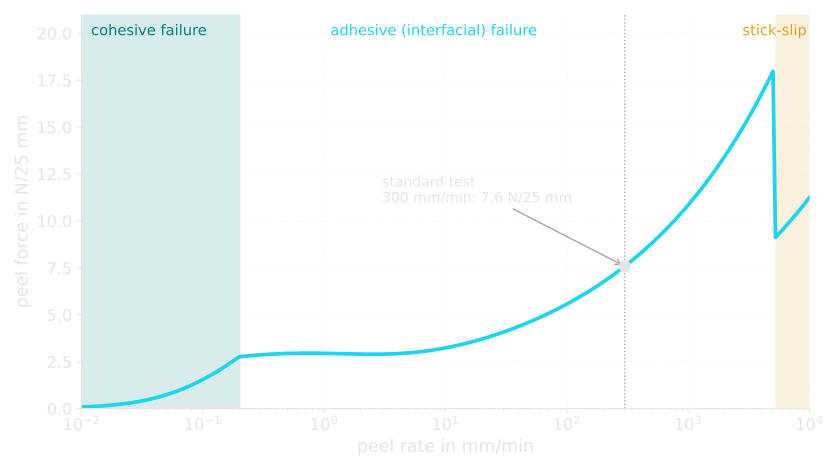
What to look for: the same tape gives very different peel forces – and even different failure modes – depending only on the speed. A single peel value always belongs to one speed and one temperature.

Try it at home – listen to the tape: Pull a strip of packaging tape off a roll very slowly: it comes off quietly and smoothly. Rip it off fast: you hear a loud “zipping” or rattling noise. That noise is stick-slip – the adhesive has become too stiff at this speed to follow smoothly and releases in tiny jerks, hundreds of times per second.

Four Ways a Tape Can Fail

The peel force alone is not enough. Users also care how the bond fails:

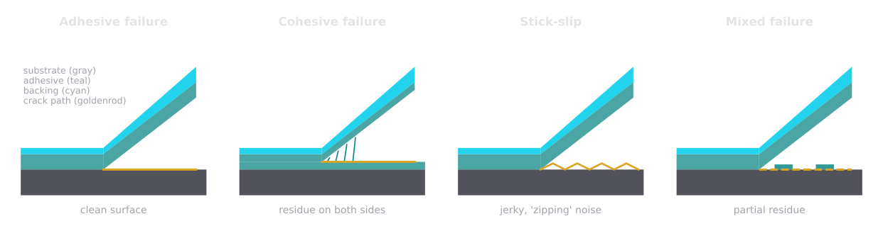
What to look for: the question is where the crack runs – along the interface, through the adhesive, or in jumps.

Failure mode	What you see	Typical rheological cause
Adhesive (interfacial)	Clean surface after peeling	Balanced adhesive, enough cohesion
Cohesive	Adhesive residue on both surfaces	Too liquid-like: low $G'$ and $\tan\delta > 1$ at slow time scales
Stick-slip	Jerky peel, zipping noise	Too stiff and glassy at the peel rate
Mixed	Partial residue	Border region between the others

For a removable label, cohesive failure is a disaster – it leaves sticky residue on the product. For a mounting tape, stick-slip means an unreliable, jerky release. A useful prediction therefore needs two answers: a number (peel force) and a category (failure mode).

Why the Chang Window Is Not Enough

In Part 8 we condensed a whole master curve into four numbers and placed the adhesive on Chang’s map. That is excellent for orientation – but it cannot deliver a peel force in N/25 mm. Four numbers at two frequencies say nothing about:

• the shape of the curves between 0.01 and 100 rad/s,
• the behavior at large deformations, when fibrils are drawn,
• the thickness of the adhesive layer and the stiffness of the backing,
• the surface, the dwell time and the test temperature.

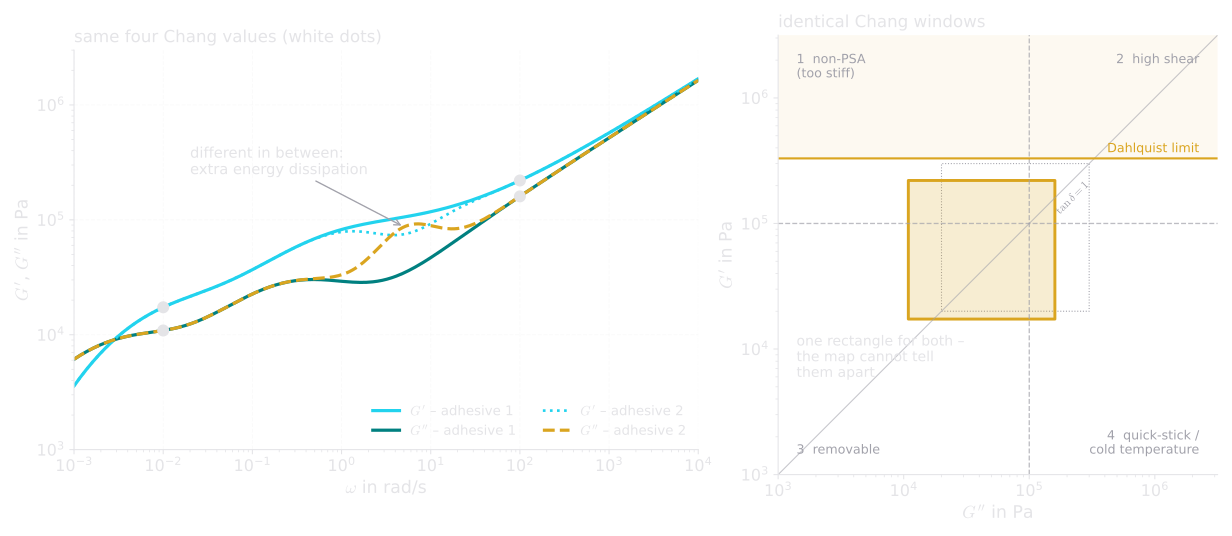
What to look for: two adhesives, one rectangle. The extra dissipation hump of adhesive 2 can change its peel force and tack noticeably – the map cannot see it.

To predict peel quantitatively, we need richer information – more “lab values” – and a method that can learn how they combine.

The Adhesive’s “Blood Values”: Rheological Features

In machine learning, the input numbers are called features. Good features are not random measurement points but quantities with a physical meaning – exactly like a doctor’s lab values. From a master curve and a temperature sweep we can read:

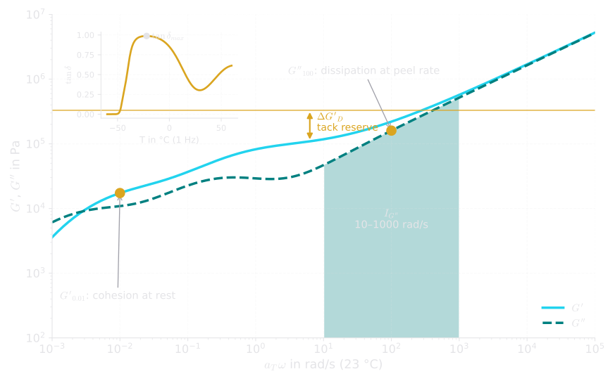
What to look for: each feature answers a physical question – how cohesive at rest, how dissipative at peel speed, how much tack reserve, where the glass transition lies.

Feature	Definition	Plain-language meaning
$G'_{0.01}$, $G''_{0.01}$	Moduli at 0.01 rad/s, 23 °C	Cohesion and flow at rest
$G'_{100}$, $G''_{100}$	Moduli at 100 rad/s	Stiffness and dissipation at peel rate
$\tan\delta_{0.01}$, $\tan\delta_{100}$	$G''/G'$ at both frequencies	Liquid-likeness at rest, damping at peel rate
$\tan\delta_{max}$, $T(\tan\delta_{max})$	Peak of a temperature sweep at 1 Hz	Damping capacity, glass transition
Loss integral $I_{G''}$	Area under $G''$ from 10 to 1000 rad/s (log axis)	Total “energy-eating capacity” at peel rates
Dahlquist margin $\Delta G'_D$	$\log_{10}\left[3.3\times10^5\ \mathrm{Pa} / G'(1\,\mathrm{Hz})\right]$	Tack reserve (above 0 = Dahlquist fulfilled)
$\eta_0$	Zero-shear viscosity (Parts 5 and 6)	Resistance to flow under a permanent load
Coat weight	Mass of adhesive per area, g/m²	Thickness of the adhesive layer

Two of these deserve a formula. The loss integral adds up the loss modulus over the range of peel frequencies:

$I_{G''} = \int_{\ln \omega_1}^{\ln \omega_2} G''\,d\ln\omega, \qquad \omega_1 = 10\ \mathrm{rad/s},\ \ \omega_2 = 1000\ \mathrm{rad/s}$

In words: instead of reading $G''$ at a single point, we measure the area under the whole $G''$ curve across the peel frequencies – the adhesive’s total capacity to “eat” energy while it is being pulled off. Integrating over $\ln\omega$ gives every decade of frequency the same weight.

The Dahlquist margin turns the tack criterion of Part 8 into a number:

$\Delta G'_D = \log_{10}\frac{3.3\times10^5\ \mathrm{Pa}}{G'(1\,\mathrm{Hz})}$

In words: how many decades softer than the Dahlquist limit the adhesive is. For Tape B, $G'(1\,\mathrm{Hz}) \approx 1.1\times10^5$ Pa, so $\Delta G'_D = \log_{10}(3) \approx 0.48$: a comfortable tack reserve. A negative value means: no tack.

Each adhesive becomes one row of such numbers, a feature vector $\mathbf{x}$ (moduli are used as logarithms). Many adhesives together form a table $X$ with $N$ rows and $p$ columns – the raw material of machine learning.

From Features to Predictions: Boosted Decision Trees

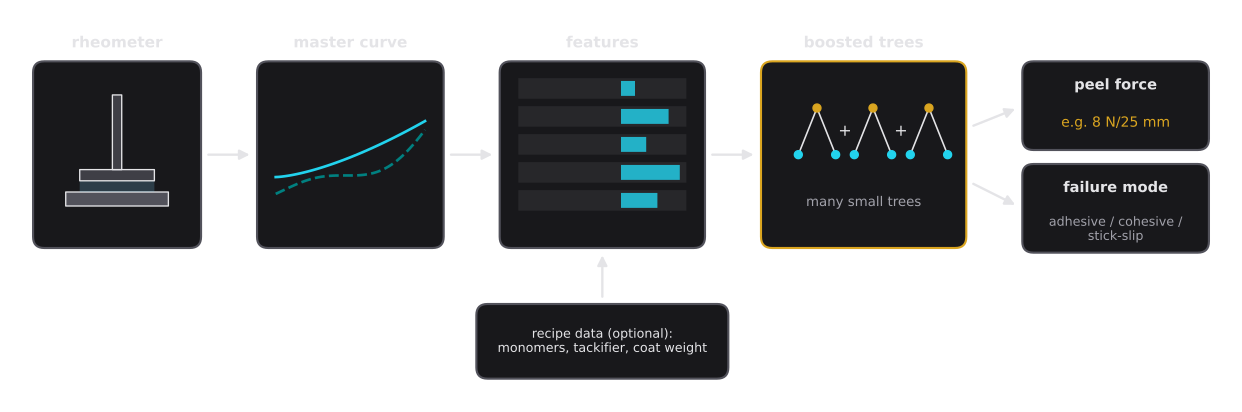
What to look for: the model never sees raw data – it sees a small table of physically meaningful numbers, and returns two answers.

One Tree: A Few Yes/No Questions

The simplest learning model that works well on such tables is the decision tree. It is nothing more than a sequence of yes/no questions – like a doctor’s diagnostic checklist: “Is $G'_{0.01}$ below $10^4$ Pa? If yes, cohesive failure is likely. If no: is $G''_{100}$ above $2\times10^5$ Pa?” Each path ends in a prediction. During training, the tree chooses the questions and thresholds that split the known examples most cleanly.

A single tree is easy to understand but crude: it can only give a few different answers, and it tends to memorize its training examples.

Many Trees: Gradient Boosting

Gradient boosting fixes this by building many small trees one after another. The first “tree” simply predicts the average peel force of all adhesives. The next tree does not try to predict the peel force itself – it predicts the error that is still left. The third tree predicts the error left after that, and so on:

$\hat{F}^{(m)}(\mathbf{x}) = \hat{F}^{(m-1)}(\mathbf{x}) + \epsilon\,h_m(\mathbf{x})$

In words: the new prediction is the old prediction plus a small correction $h_m$ from the next tree. The learning rate $\epsilon$ (for example 0.05) makes each correction deliberately small, so that no single tree can dominate – the model improves in many careful steps.

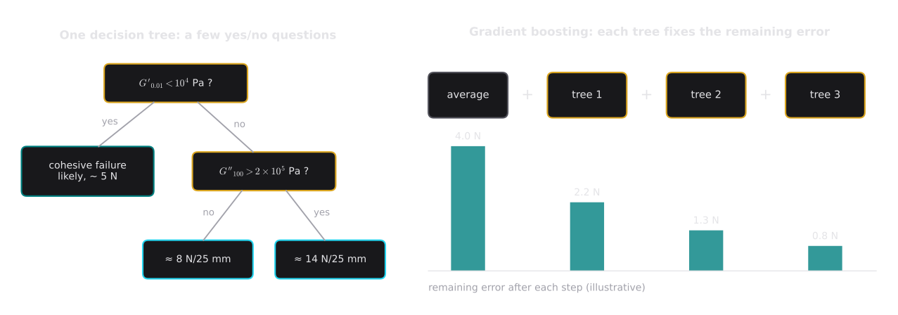
What to look for: each tree is weak on its own. Together, each one cleaning up after the others, they become a strong predictor.

Everyday example – a team of apprentices: Imagine estimating the weight of parcels. The first apprentice simply guesses the average. The second looks at the first one’s mistakes and learns a simple rule: “big boxes are heavier than guessed”. The third corrects what is still wrong: “boxes marked ‘books’ are heavier still”. None of them is an expert – but the sum of their corrections becomes surprisingly accurate. That is gradient boosting. Popular implementations are XGBoost, LightGBM and the histogram-based gradient boosting in scikit-learn, which we use here.

What does “error” mean exactly? For the peel force (a regression), the model minimizes the mean squared error:

$L = \frac{1}{N}\sum_{i=1}^{N}\left(F_{peel,i} - \hat{F}_{peel,i}\right)^2$

For the failure mode (a classification), it minimizes the cross-entropy:

$L_{CE} = -\frac{1}{N}\sum_{i=1}^{N}\sum_{k=1}^{K} y_{ik}\,\log\hat{p}_{ik}$

In words: the model predicts a probability $\hat{p}_{ik}$ for each of the $K$ failure modes; $y_{ik}$ is 1 for the true mode and 0 otherwise. The model is punished most when it is confident about the wrong answer. To avoid memorizing noise, the trees are kept small (here at most 15 leaves each) and large correction values are penalized – a built-in preference for simple explanations.

A Transparent Test Case: 300 Virtual Adhesives

To demonstrate the method openly, we need data – and real, published data sets that combine full rheology with standardized peel tests are rare. We therefore built a synthetic data set whose rules are fully known. Every step is described here, so that nothing is hidden:

Step	What happens	Range / rule
1 Recipe	300 virtual acrylic adhesives	2-ethylhexyl acrylate with 0–15 % methyl methacrylate, 0–8 % acrylic acid, 0–45 phr tackifier resin, crosslinker level 0–1, molar mass ×0.25 to ×4, coat weight 15–60 g/m²
2 Glass transition	Fox equation $1/T_g = \sum_j w_j / T_{g,j}$	Monomer and resin $T_g$ values from literature
3 Rheology	Multimode Maxwell spectrum, shifted with WLF according to $T_g$	Tackifier dilutes the plateau, crosslinker adds a network
4 Features	Read from the model master curve and temperature sweep	All features of the table above; ~5 % rheometer repeatability
5 Peel force	Gent–Schultz-type rule: tack factor × $[1 + (G''_{peel}/G_{ref})^{0.7}]$ × thickness factor	Peel frequency $\omega \approx v/h$; ~7 % test scatter
6 Failure mode	Cohesive if the adhesive’s cohesive strength (from $G'$ at the slower fibril time scale) is lower than the interfacial peel force; stick-slip if $G' > 10^6$ Pa at the peel frequency	5 % of labels deliberately randomized

Each virtual adhesive was “tested” three times, as in a real lab: 900 rows in total. About 74 % of them fail adhesively, 12 % cohesively and 14 % by stick-slip.

Honesty box – read this first: A model trained on synthetic data learns the rules of the data generator – not the laws of nature. Everything below demonstrates the method: which features to use, how to train, how to validate, how to use a model for decisions. It does not prove that real adhesives follow these rules. A model you can trust needs measured data – realistically 100 or more formulations with full rheology and standardized peel tests – and must be checked on lab data it has never seen.

Honest Validation: Did the Model Really Learn Something?

A model that has memorized its examples can look perfect on them and fail completely on anything new. Good validation is therefore at least as important as the model itself. Three rules:

1. Keep a test set aside. 20 % of the adhesives (60 recipes, 180 rows) never take part in training. Only at the very end is the model allowed to predict them.
2. Split by recipe, not by row. The three repeat tests of one adhesive are almost identical. If one repeat ended up in training and another in the test set, the model could simply “recognize” the adhesive. All repeats of a recipe therefore stay together – grouped splitting.
3. Cross-validate. Within the training data, the model is trained five times on four fifths and checked on the remaining fifth (again grouped). The spread of these five results shows how stable the model is.

Peel Force: The Parity Plot

The most honest picture of a regression model is the parity plot: predicted value against measured value for every test adhesive. A perfect model would put every point on the diagonal.

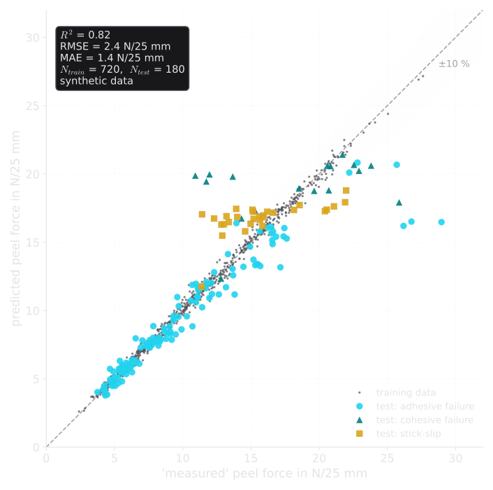
What to look for: most test points hug the diagonal. The outliers are almost all adhesives close to a change of failure mode – where a small change in the recipe makes the peel force jump.

Three numbers summarize the plot:

• $R^2 = 0.82$: the model explains 82 % of the variation in peel force between adhesives. Grouped cross-validation gives a similar $R^2 = 0.86 \pm 0.07$ – the result is stable.
• MAE = 1.4 N/25 mm: the typical (mean absolute) error.
• RMSE = 2.4 N/25 mm: the root-mean-square error, which weighs large misses more heavily. That it is clearly larger than the MAE shows that the error is not spread evenly: a few adhesives near a failure-mode boundary cause most of it.

Failure Mode: The Confusion Matrix

For the failure mode, the confusion matrix counts how often each true mode was predicted as which mode:

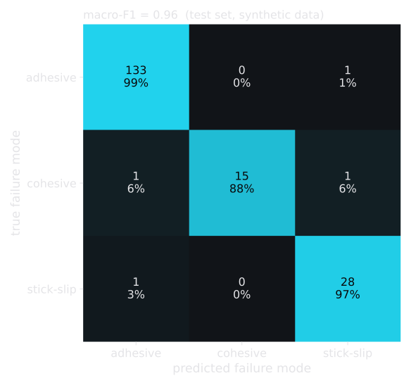
What to look for: the diagonal holds almost all cases. The weakest class is cohesive failure – it is also the rarest, so the model has seen the fewest examples.

The macro-F1 score of 0.96 averages precision and recall over all three classes equally, so a rare class like cohesive failure counts as much as the frequent adhesive failure. Remember that 5 % of the labels were deliberately scrambled: a perfect score would actually be suspicious.

Which Lab Values Matter?

A model that predicts well is useful; a model that also shows why is valuable. A simple, robust method is permutation importance: shuffle the values of one feature across all test adhesives – destroying its information – and see how much worse the predictions become.

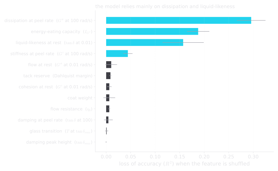
What to look for: the model relies on dissipation at peel speed – exactly what Gent and Schultz predicted – and on liquid-likeness at rest, which decides about cohesive failure.

The ranking makes physical sense: dissipation drives the peel force, and liquid-likeness at slow time scales decides whether the adhesive tears internally. Two cautions:

• Correlated features share their importance. $G''_{100}$ and the loss integral carry similar information; shuffling one hurts less because the other remains. A low importance does not mean a feature is useless.
• The model can only find what is in the data. $\tan\delta_{max}$ scores near zero here because our generator’s peel rule does not use it directly. With real data, the ranking may look quite different – and that is exactly what makes a real study interesting.

For explanations of individual predictions (“why does the model expect 15 N for this recipe?”), methods such as SHAP values split each prediction into contributions of the individual features.

The What-If Map: Rheology as a Formulation Tool

A trained model becomes most useful when we ask it questions. Keep a base recipe, vary two ingredients – here the tackifier (0–45 phr) and the crosslinker – compute the rheology of each virtual variant, and let the models predict peel force and failure mode. Plotted on two Chang axes, the result is a map:

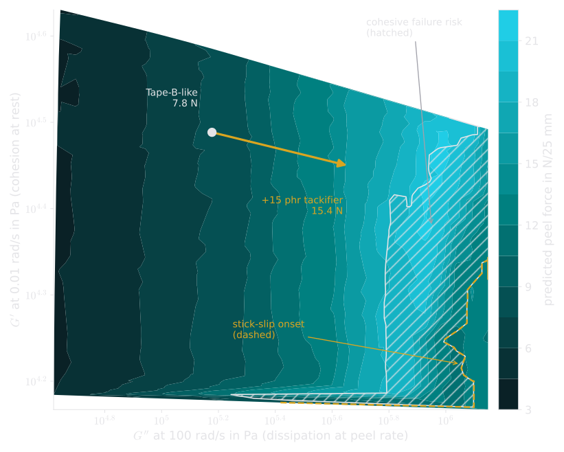
What to look for: moving right (more dissipation) raises the peel force – but too far, and the adhesive enters the hatched zone where it starts to fail cohesively and leave residue.

Worked example. A virtual adhesive close to our Tape B (15 phr tackifier) is predicted at 7.8 N/25 mm with adhesive failure. Adding another 15 phr of tackifier moves it to the right and slightly down – just as the formulation arrows of Part 8 predicted – and doubles the predicted peel force to 15.4 N/25 mm. But the new point lies close to the cohesive-risk zone: a formulator would now check whether the adhesive still releases cleanly, or add a little crosslinker to move it back up.

We can also run the model on the three tapes of this series, whose master curves it has never seen: it predicts 3.7, 6.9 and 12.8 N/25 mm for Tapes A, B and C, close to the values the generator’s rules assign to them (3.5, 7.6 and 13.0 N/25 mm), all with adhesive failure. The ranking – removable label, general-purpose tape, mounting tape – is the same as in every previous part.

How Much Data Does It Take?

The final question for anyone planning a real project: how many adhesives must be measured? A learning curve answers it: train the model on growing numbers of recipes and measure the test error each time.

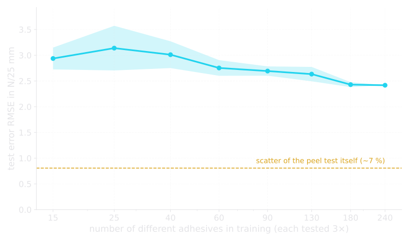
What to look for: more adhesives help, but the curve flattens. The gap to the dashed line – the scatter of the peel test itself – comes from adhesives near failure-mode boundaries, which need many more examples.

Two practical lessons follow. First, no model can be more precise than the test it learns from: the peel test’s own scatter (here about 7 %, in practice often 5–15 %) is a hard floor. Second, the difficult cases are the interesting ones – adhesives close to cohesive failure or stick-slip. A real data set should deliberately include such borderline formulations instead of only “good” products.

In the lab – building a real data set:

• Use one rheology protocol for all samples: same geometries, temperatures, frequencies and strain inside the LVE range (Part 7), with master curves at 23 °C (Part 8).
• Test peel with one standard (for example FINAT FTM 1, 180°, 300 mm/min), one substrate and fixed dwell times; record the failure mode for every strip.
• Measure at least three strips per adhesive and keep them together as a group when splitting the data.
• Record the recipe and the coat weight – they are cheap features and help the model.
• Before trusting a model, test it on a batch of new formulations it has never seen.

Why It Matters for Adhesives

This series began with honey and water and ends with machine learning – but the thread is the same throughout. Every part added one way of asking a material how it responds to force and time: flow curves, creep, relaxation, oscillation, master curves. The Chang window turned those answers into a map. A machine-learning model, trained on good data, turns the map into a forecast: peel force and failure mode from an afternoon of rheology, instead of days of coating and testing.

The physics does not disappear in the model – it is the reason the model works. The features that matter are the ones rheology told us to look at: dissipation at peel speed, liquid-likeness at rest, tack reserve. Machine learning does not replace understanding; it rewards it.

Key Takeaways

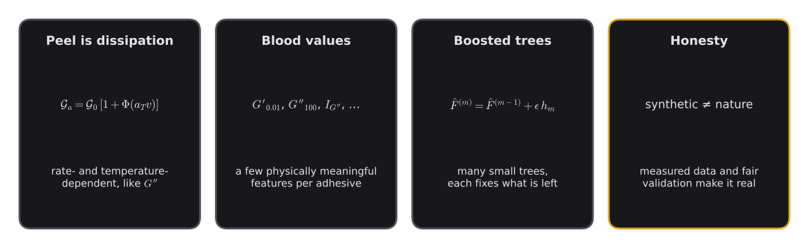
• Peel strength is mostly viscoelastic dissipation; it depends on speed and temperature like $G''$ (Gent–Schultz).
• A useful prediction has two parts: the peel force in N/25 mm and the failure mode (adhesive, cohesive, stick-slip).
• The Chang window is an excellent map, but four numbers are not enough – richer rheological features such as the loss integral and the Dahlquist margin carry more information.
• Gradient-boosted trees learn from such features step by step, each small tree correcting the remaining error.
• Honest validation – a separate test set, grouped splits, parity plots, confusion matrices – is as important as the model.
• What-if maps turn a trained model into a formulation tool – but only measured data make it trustworthy.

Key Terms

Term	Meaning in plain language	Symbol, unit
Peel force	Force to pull a tape off, per width	$F/b$, N/25 mm
Peel energy	Work to separate one square meter of bond	$\mathcal{G}_a$, J/m²
Stick-slip	Jerky peel with alternating sticking and sudden release	–
Cohesive failure	Crack runs through the adhesive, leaving residue	–
Feature	One input number describing an adhesive	$x_j$
Loss integral	Area under $G''$ over the peel frequencies	$I_{G''}$, Pa
Dahlquist margin	Tack reserve in decades	$\Delta G'_D$, –
Decision tree	Chain of yes/no questions ending in a prediction	–
Gradient boosting	Many small trees, each correcting the remaining error	$\hat{F}^{(m)}$
Learning rate	How large each correction step is	$\epsilon$
Test set	Data kept aside to check the finished model	–
Grouped split	Keeping repeats of one recipe together	–
$R^2$, RMSE, MAE	Share of explained variation; typical errors	–, N/25 mm
Confusion matrix	Table of true vs. predicted categories	–
Permutation importance	Loss of accuracy when a feature is shuffled	–

The End of the Series – and a Beginning

Over nine parts, we have gone from the two-plate model to machine learning: from why honey flows more slowly than water (Part 1) to how a rheometer measures it (Part 2), from springs (Part 3) and dashpots to viscoelasticity (Part 4), creep (Part 5), relaxation (Part 6) and oscillation (Part 7), and finally to the Chang window (Part 8) and peel prediction. The next step is not another article – it is real data. If you measure adhesives, you now have a recipe for turning your rheometer into a forecasting tool.

Two interactive bonus parts let you watch a rheometer at work: in Part 10 you measure the flow curve of water in a bob-and-cup geometry, in Part 11 a frequency sweep of an acrylic adhesive.

References

1. Gent, A. N.; Schultz, J.: Effect of wetting liquids on the strength of adhesion of viscoelastic material, The Journal of Adhesion 3 (1972) 281–294.
2. Chang, E. P.: Viscoelastic windows of pressure-sensitive adhesives, The Journal of Adhesion 34 (1991) 189–200.
3. Creton, C.: Pressure-sensitive adhesives: an introductory course, MRS Bulletin 28 (2003) 434–439.
4. Fox, T. G.: Influence of diluent and of copolymer composition on the glass temperature of a polymer system, Bulletin of the American Physical Society 1 (1956) 123.
5. Friedman, J. H.: Greedy function approximation: a gradient boosting machine, The Annals of Statistics 29 (2001) 1189–1232.
6. Chen, T.; Guestrin, C.: XGBoost: a scalable tree boosting system, Proceedings of the 22nd ACM SIGKDD Conference (2016) 785–794.
7. Lundberg, S. M.; Lee, S.-I.: A unified approach to interpreting model predictions, Advances in Neural Information Processing Systems 30 (2017).
8. Pedregosa, F. et al.: Scikit-learn: machine learning in Python, Journal of Machine Learning Research 12 (2011) 2825–2830.
9. FINAT: FINAT Test Method No. 1 – Peel Adhesion (180°) at 300 mm per Minute, FINAT Technical Handbook, The Hague.