8 The Chang Viscoelastic Window: A Map for Pressure-Sensitive Adhesives
Why does a sticky note come off cleanly while packaging tape holds for months – and why does a tape from the freezer not stick at all? An illustrated introduction to the Dahlquist criterion, time–temperature superposition and Chang's viscoelastic window.
A sticky note comes off cleanly and can be stuck on again somewhere else. Packaging tape holds a heavy box closed for months. A plaster must stay on your skin all day and still come off without hurting. A freezer label has to grab a frozen bag at −20 °C. And a double-sided mounting pad carries a picture hook for years.
All of these are pressure-sensitive adhesives (PSAs): they stick on contact, with nothing more than light pressure – no water, no heat, no curing. Yet each one needs a different balance. When you press it on, an adhesive must behave like honey and flow into the surface. When you pull it off, it must resist like leather. How can one material be both – and how can you tell, from a rheometer measurement, which job an adhesive is good for?
In the 1990s, Eric P. Chang at Avery Dennison answered this with a remarkably simple tool: the viscoelastic window. It condenses the frequency sweep of Part 7 into four numbers and places the adhesive on a map. This article builds that map step by step.
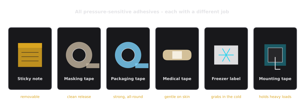
What to look for: six products, six different jobs – but the same basic material class. The differences lie almost entirely in their viscoelastic behavior.
One Material, Two Time Scales
Every use of a tape consists of two very different moments:
- Bonding is slow. When you press a tape onto cardboard, the adhesive has seconds to minutes to flow into the tiny hills and valleys of the surface. Only where it touches does it stick. To do this, it must be soft and liquid-like – a low storage modulus .
- Debonding is fast. When you pull the tape off, the adhesive in the peel zone is stretched within milliseconds. It forms fine threads, the fibrils, which stretch, dissipate energy and finally snap. The more energy is lost on the way, the harder it is to peel. For this, the adhesive needs a high loss modulus at high speed.
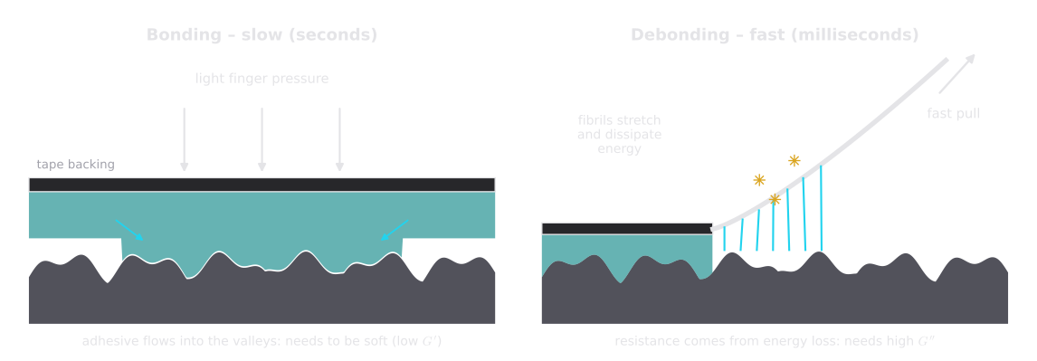
What to look for: bonding and debonding happen on time scales that differ by a factor of about ten thousand. The same adhesive faces two completely different tasks.
This is the Deborah number of Part 4 in action: during slow bonding, the adhesive has time to flow ( small, liquid-like); during fast peeling, it has no time ( large, solid-like). And in Part 7 we learned how to translate time into frequency: .
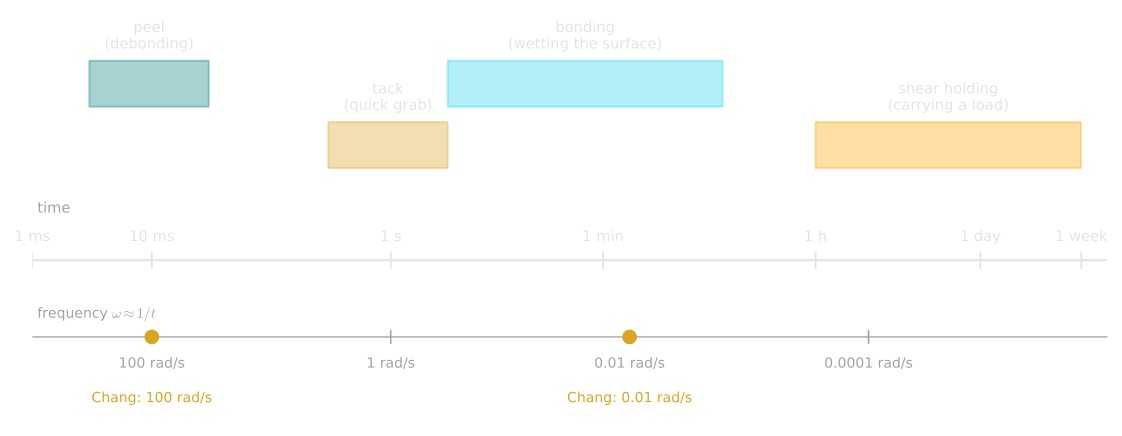
What to look for: each adhesive process has its own time scale – and therefore its own frequency. The two goldenrod dots are the frequencies Chang chose as representatives of debonding and bonding.
| Process | Everyday meaning | Time scale | Frequency proxy | What the adhesive needs |
|---|---|---|---|---|
| Peel / debonding | Pulling the tape off | ≈ 10 ms | rad/s | High – lots of energy dissipation |
| Tack | Quick grab on light contact | ≈ 1 s | 1 Hz = 6.28 rad/s | below the Dahlquist limit |
| Bonding / wetting | Pressing the tape on | seconds – minutes | rad/s | Low – soft enough to flow into roughness |
| Shear holding | Carrying a load for days | hours – days | rad/s | Enough , little flow – cohesion |
Worked example – why 100 rad/s? A standard peel test pulls the tape off at 300 mm/min, that is 5 mm/s. The adhesive layer is typically 25 µm thick. In the peel zone, the adhesive is therefore sheared at roughly – the same order of magnitude as an oscillation at 100 rad/s.
Try it at home – fast vs. slow peel: Stick a strip of packaging tape on a cardboard box and peel it off very slowly: it often comes off cleanly with little force. Stick on another strip and rip it off quickly: it is much harder, and it may tear the top layer of the cardboard. Same tape, same box – only the speed, and with it the frequency, has changed.
The Dahlquist Criterion: Soft Enough to Grab
Before an adhesive can hold anything, it has to make contact. Put a tape on a surface without pressing: does it grab? This quick stickiness is called tack. In the 1960s, Carl Dahlquist of 3M found a remarkably simple rule for it: an adhesive is only tacky if it is soft enough within about one second of contact.
Dahlquist originally formulated the rule as a creep compliance: must exceed about – the value we used for the tapes in Part 5. Today it is usually expressed as a storage modulus at 1 Hz:
In words: an adhesive only grabs on light contact if, at the time scale of a touch, it is softer than about a third of a megapascal – softer than a rubber band. Stiffer materials cannot deform quickly enough into the roughness of a surface; they touch only at a few high points and fall off.
The exact number varies between sources – values between about 0.1 MPa (the strict inverse of Dahlquist’s compliance) and 0.33 MPa are common; Mezger’s handbook gives 0.33 MPa. In this series we use Pa as the line on the map.
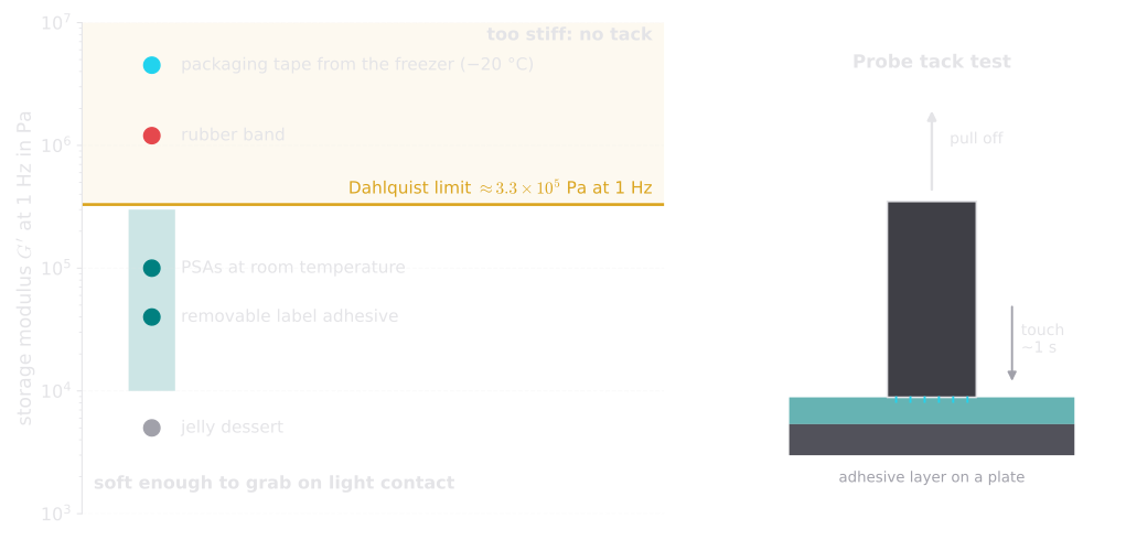
What to look for: all room-temperature PSAs sit just below the line – soft, but not too soft. A tape from the freezer jumps far above it.
Common pitfall – necessary, not sufficient: Fulfilling Dahlquist only means that an adhesive can make contact. A jelly dessert is far below the line and still makes a very poor adhesive: it has no strength to resist when you pull. Good adhesion needs softness for bonding and dissipation and cohesion for debonding and holding – which is exactly why Chang looked at more than one number.
Time–Temperature Superposition: Colder Is Faster
To build a Chang window, we need and at 0.01 rad/s and at 100 rad/s. The first is slow – one cycle takes more than ten minutes. The second is fine for most rheometers. But the high-frequency behavior of adhesives that matters in peeling reaches far beyond 100 rad/s, and no rotational rheometer can oscillate at a million rad/s. The solution is a clever trick: instead of making the measurement faster, we make the material slower – by cooling it.
The idea is called time–temperature superposition (TTS). In a polymer, all relaxation processes depend on the mobility of the chains, and this mobility changes with temperature. When you cool a polymer, every inner motion slows down by the same factor. For the material, a deformation at a given speed therefore looks faster than it would at room temperature. Cooling has the same effect as speeding up – colder is faster.
Everyday example – honey in the fridge: Stir cold honey from the fridge and it feels stiff and resists like a much thicker substance. Warm it up and it runs off the spoon. You did not change the honey – only its “inner clock”. For polymers, this clock is so reliable that a temperature change can replace a change of speed by many orders of magnitude.
In practice, frequency sweeps are measured at several temperatures – for example from −40 °C to +80 °C in steps of 20 K – each over the comfortable range of 0.1 to 100 rad/s. Then each curve is shifted horizontally along the frequency axis until they all join into a single master curve at a chosen reference temperature :
In words: the modulus measured at temperature and frequency equals the modulus at the reference temperature at the “reduced” frequency . The shift factor tells how many times faster (cold, ) or slower (warm, ) the material “lives” at compared with .
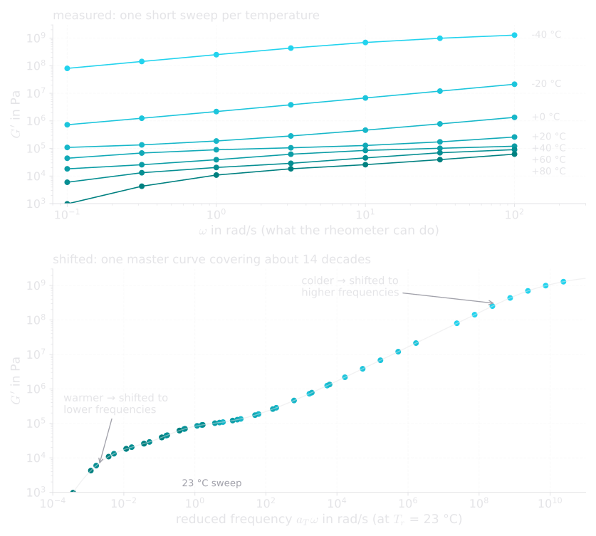
What to look for: seven short pieces become one long curve – like pieces of a puzzle. A single measurement at 23 °C (shaded band) would show only a tiny part of it.
The WLF Equation
How large is the shift? For polymers above their glass transition temperature , the shift factors follow the WLF equation, named after Williams, Landel and Ferry (1955):
In words: the further the temperature is from the reference, the larger the shift – but not symmetrically. Close to the glass transition (cold side), a few kelvin change the speed by orders of magnitude; far above it (warm side), the effect is milder. and are material constants.
Worked example. For an acrylic PSA with °C, the “universal” WLF constants converted to °C give and K. At °C ( K):
A sweep from 0.1 to 100 rad/s at −17 °C therefore corresponds to 600 to 600,000 rad/s at room temperature. At °C, – the same sweep reaches down to 0.0013 rad/s. That is how both Chang frequencies become accessible within one afternoon of measuring.
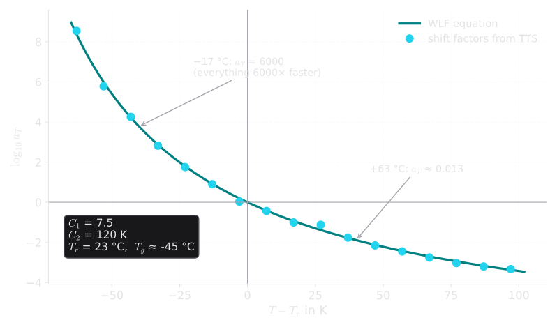
What to look for: the curve is steep on the cold side and flat on the warm side. Just 40 K of cooling speed the material up by a factor of several thousand.
In the lab – when TTS works, and when it does not: TTS assumes that all relaxation processes speed up or slow down by the same factor – the material is “thermorheologically simple”. This fails when the structure changes with temperature: crystallization, melting of hard domains in block-copolymer adhesives, phase separation of a tackifier. A quick check is the van Gurp–Palmen plot, the phase angle versus : it does not use the frequency at all, so the data of all temperatures must fall on one curve if TTS is valid.
Reading the Master Curve
Here is the master curve of our general-purpose Tape B at 23 °C – the same model adhesive we followed through creep (Part 5), relaxation (Part 6) and oscillation (Part 7), now completed with its fast processes:
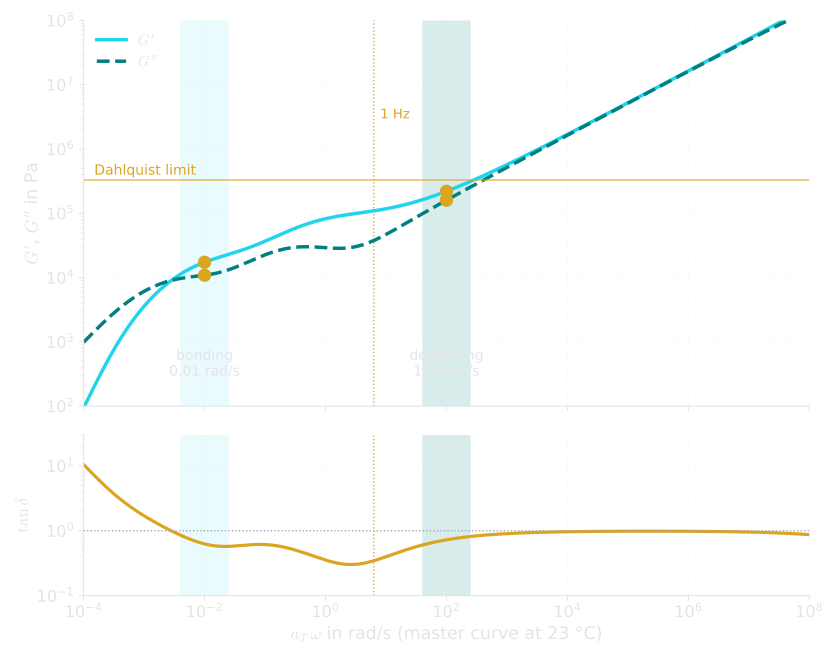
What to look for: at 0.01 rad/s the adhesive is soft and fairly liquid-like; at 100 rad/s it is stiffer and dissipates much more energy ( has caught up with ). At 1 Hz, stays below the Dahlquist line.
From this curve we read:
| Quantity | Tape B (model data) |
|---|---|
| at 0.01 rad/s | ≈ Pa |
| at 0.01 rad/s | ≈ Pa |
| at 100 rad/s | ≈ Pa |
| at 100 rad/s | ≈ Pa |
| at 1 Hz | ≈ Pa – Dahlquist fulfilled |
Building the Chang Window in Four Steps
Chang’s idea is to plot these values not over frequency, but against each other: storage modulus on the vertical axis, loss modulus on the horizontal axis, both logarithmic. The recipe:
- Measure the frequency sweep at room temperature – directly or via TTS.
- Read four values: , , and .
- Draw the rectangle in the – plane with the corners and . The other two corners combine the values “crosswise”.
- Place it on the map and see in which region it lies.
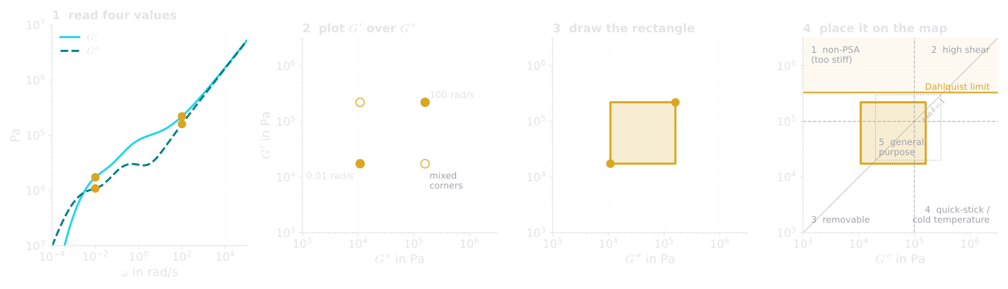
What to look for: the lower-left corner is the bonding behavior (slow), the upper-right corner the debonding behavior (fast). The rectangle between them is the adhesive’s “window” of use.
The Map: Five Regions
Chang divided the – plane into four quadrants and a central region. Each stands for a family of adhesives:
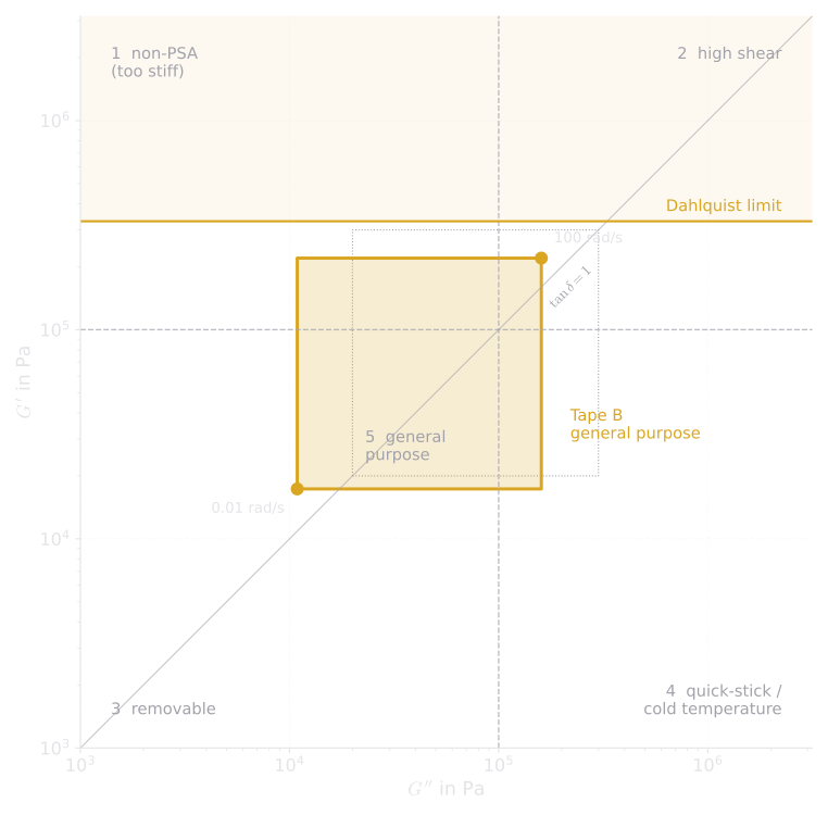
What to look for: Tape B’s window sits in the middle of the map and below the Dahlquist line – a balanced, general-purpose adhesive. The region boundaries are drawn schematically at about Pa; different publications place them slightly differently.
| Region | Position on the map | Adhesive type | Everyday example | ||
|---|---|---|---|---|---|
| 1 | high | low | upper left | Non-PSA – too stiff, no tack | Plastic film, release coating |
| 2 | high | high | upper right | High-shear PSA | Mounting tape |
| 3 | low | low | lower left | Removable PSA | Sticky note, removable label, medical tape |
| 4 | low | high | lower right | Quick-stick / cold-temperature PSA | Freezer label |
| 5 | medium | medium | center | General-purpose PSA | Packaging tape |
The logic behind the map is easy to remember:
- Up (higher ) means more elastic, more cohesive – better shear holding, but less tack.
- Right (higher ) means more dissipation – higher peel forces and quick grab.
- Down and left means soft and weak – easy to remove.
- The diagonal separates solid-like behavior (above) from liquid-like behavior (below).
Quick check: An adhesive has Pa, Pa, Pa and Pa. Where is its window? (All values are well below Pa: lower left – a removable adhesive.)
Three Tapes and a Freezer Label
Now let us place the three model tapes of this series on the map, together with an illustrative freezer label:
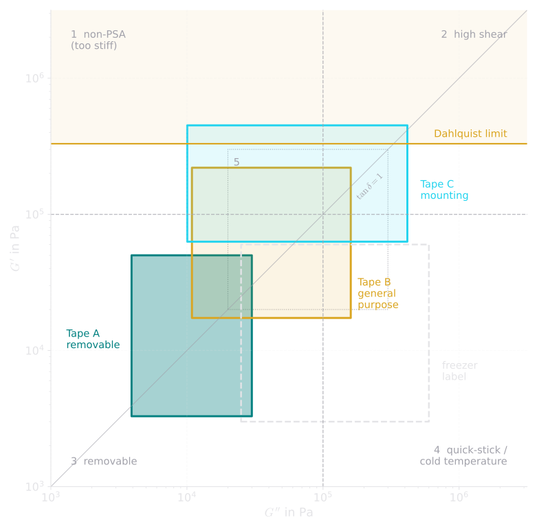
What to look for: the three tapes that behaved so differently in the creep test of Part 5 now land in three different regions of the map – the ranking is the same.
| Tape (model data) | (1 Hz) | Region | ||||
|---|---|---|---|---|---|---|
| A – removable label | 3,300 Pa | 3,900 Pa | 50,000 Pa | 30,000 Pa | 33 kPa | 3 – removable |
| B – general purpose | 17,000 Pa | 11,000 Pa | 220,000 Pa | 160,000 Pa | 110 kPa | 5 – general purpose |
| C – high-shear mounting | 63,000 Pa | 10,000 Pa | 450,000 Pa | 420,000 Pa | 140 kPa | towards 2 – high shear |
Two details are worth a closer look:
- Tape A has at 0.01 rad/s: at slow time scales it is liquid-like. That is why it wets a surface easily and comes off cleanly – and why it slowly creeps off under a permanent load (0.3 hours holding time in Part 5).
- Tape C’s window reaches above the Dahlquist line at 100 rad/s. That is not a contradiction: the Dahlquist criterion refers to 1 Hz, where Tape C is still soft enough (140 kPa). But it is only just soft enough – mounting tapes usually need firm pressure to bond.
How Formulation Moves the Window
The real strength of the Chang window is that it turns rheology into a formulation tool. The main ingredients of a PSA move the window in predictable directions:
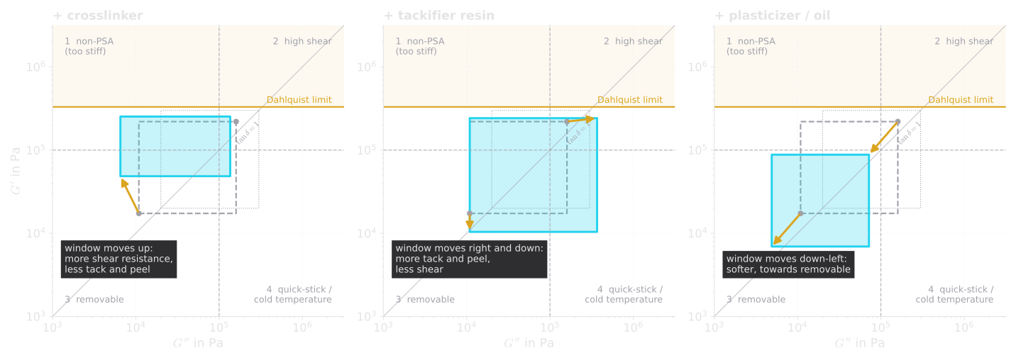
What to look for: each ingredient pushes the window in its own direction. A formulator combines them to steer the window into the region the product needs.
- Crosslinker: additional chemical bonds between the chains act like a permanent network. at low frequency rises, at low frequency falls – the window moves up: better shear holding and heat resistance, but less tack and peel. Too much, and the window leaves the region of good PSAs altogether.
- Tackifier resin: a low-molecular-weight resin with a high glass transition temperature. It raises the of the mixture and dilutes the entanglements. at high frequency rises strongly, at low frequency falls – the window moves right and down: more tack and peel, less shear.
- Plasticizer or oil: it softens everything. Both moduli drop at all frequencies – the window moves down and left, towards the removable region.
Why Your Tape Fails in the Freezer
With time–temperature superposition, the Chang window can also answer a question everyone has experienced: why does a normal tape not stick in the cold? Cooling makes the adhesive “faster” – so at −20 °C the window of Tape B is simply its 23 °C master curve read at frequencies times higher.
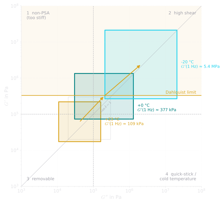
What to look for: cooling moves the whole window up and to the right. At 0 °C, Tape B just reaches the Dahlquist limit; at −20 °C it is more than ten times too stiff to grab.
Worked example. With the WLF constants above, at 0 °C and at −20 °C. The tack frequency of 1 Hz at −20 °C therefore corresponds to rad/s on the 23 °C master curve – deep in the transition zone, where MPa. The tape feels like a plastic film.
A real freezer label solves this with a much lower glass transition temperature and more “liquid” character: its window sits low and far to the right at room temperature, so that even after the shift into the cold it stays below the Dahlquist line.
Try it at home – cold tape: Put a roll of packaging tape in the freezer for an hour. Take it out and try to stick a strip on a box: it hardly grabs, and the adhesive feels hard and smooth. Warm the strip between your hands for a minute and try again – it sticks as usual. You have just moved an adhesive across the Dahlquist line and back.
In the lab – measuring a Chang window: For adhesives, parallel plates of 8 mm (cold, stiff) and 25 mm (warm, soft) are typical, with a sample thickness of about 1 mm made from several laminated layers. Measure frequency sweeps from 100 to 0.1 rad/s at temperatures from about −40 °C to +120 °C in steps of 10 K, always with a strain inside the LVE range (check with an amplitude sweep at the coldest and the warmest temperature). Build the master curve at 23 °C, check it with a van Gurp–Palmen plot, then read the four values.
Why It Matters for Adhesives
The Chang window is popular in the adhesives industry because it is simple: four numbers from a standard measurement, one rectangle, one map. It lets a formulator compare a new adhesive with an existing product, see at a glance whether it will be tacky, and decide which ingredient to change.
It also has limits. The map uses only two frequencies and says nothing about the substrate, the thickness of the adhesive layer or the backing – all of which change peel forces considerably. And the boundaries between the regions are a guide, not a law. For quantitative predictions, more of the master curve has to be used – which is exactly what the machine-learning approach of the next part does.
Key Takeaways
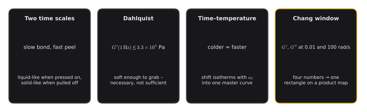
- A PSA must be soft and liquid-like when pressed on (slow) and tough and dissipative when peeled off (fast) – one material, two time scales.
- Dahlquist: Pa is required for tack – necessary, but not sufficient.
- Time–temperature superposition (“colder = faster”) gives access to frequencies no single measurement can reach; the WLF equation describes the shift.
- Chang’s window condenses a frequency sweep into four numbers – and at 0.01 and 100 rad/s – and places the adhesive on an application map with five regions.
- Crosslinker moves the window up, tackifier right and down, plasticizer down and left – rheology becomes a formulation tool.
- Cooling moves the window up and to the right – that is why an ordinary tape does not stick in the freezer.
Key Terms
| Term | Meaning in plain language | Symbol, unit |
|---|---|---|
| Pressure-sensitive adhesive (PSA) | Adhesive that sticks on light contact, without curing | – |
| Tack | Quick grab on light, short contact | – |
| Fibrils | Fine threads of adhesive formed during peeling | – |
| Dahlquist criterion | Upper stiffness limit for tack | Pa |
| Time–temperature superposition (TTS) | Replacing a change of speed by a change of temperature | – |
| Shift factor | How many times faster the material “lives” at | , – |
| WLF equation | Formula for the shift factor above | , |
| Master curve | All isotherms shifted into one curve at | – |
| van Gurp–Palmen plot | Phase angle over – check for valid TTS | – |
| Chang viscoelastic window | Rectangle from , at 0.01 and 100 rad/s | Pa |
| Crosslinker | Creates permanent bonds between chains | – |
| Tackifier | Resin that raises and tack | – |
| Plasticizer | Oil or additive that softens the adhesive | – |
Coming Up Next
A doctor does not wait for symptoms: a handful of lab values already tells a lot about your health. In the same way, a few rheological “lab values” of an adhesive – measured in minutes – can predict how strongly a tape will stick and how it will fail, before a single peel test is run. In Part 9, the final part of this series, we turn the master curve into features for a machine-learning model that predicts peel adhesion.
References
- Chang, E. P.: Viscoelastic windows of pressure-sensitive adhesives, The Journal of Adhesion 34 (1991) 189–200.
- Chang, E. P.: Viscoelastic properties of pressure-sensitive adhesives, The Journal of Adhesion 60 (1997) 233–248.
- Dahlquist, C. A.: Tack, in: Adhesion Fundamentals and Practice, Maclaren, London 1969, pp. 143–151.
- Williams, M. L.; Landel, R. F.; Ferry, J. D.: The temperature dependence of relaxation mechanisms in amorphous polymers and other glass-forming liquids, Journal of the American Chemical Society 77 (1955) 3701–3707.
- Van Gurp, M.; Palmen, J.: Time–temperature superposition for polymeric blends, Rheology Bulletin 67 (1998) 5–8.
- Creton, C.: Pressure-sensitive adhesives: an introductory course, MRS Bulletin 28 (2003) 434–439.
- Mezger, T. G.: The Rheology Handbook, 5th ed., Vincentz Network, Hanover 2020.
- Ferry, J. D.: Viscoelastic Properties of Polymers, 3rd ed., Wiley, New York 1980.