5 Creep and Creep Recovery: How Materials Deform Under Constant Load

You tape a poster to the wall in the evening. The next morning it hangs a few centimeters lower than before. Nobody pulled on it – only its own weight acted, gently and constantly, all night long. When you take the poster down and look at the tape, part of its deformation springs back; another part is gone for good.

This slow deformation under a constant load is called creep. It is everywhere once you start looking: a bookshelf that sags a little more every year, a memory-foam mattress that keeps the shape of your body for a while after you get up, a car tire with a flat spot after a winter in the garage. In Part 4 we learned that viscoelastic materials behave like solids on short time scales and like liquids on long ones. A creep test is the rheologist’s way of watching this over time – and of turning it into numbers.

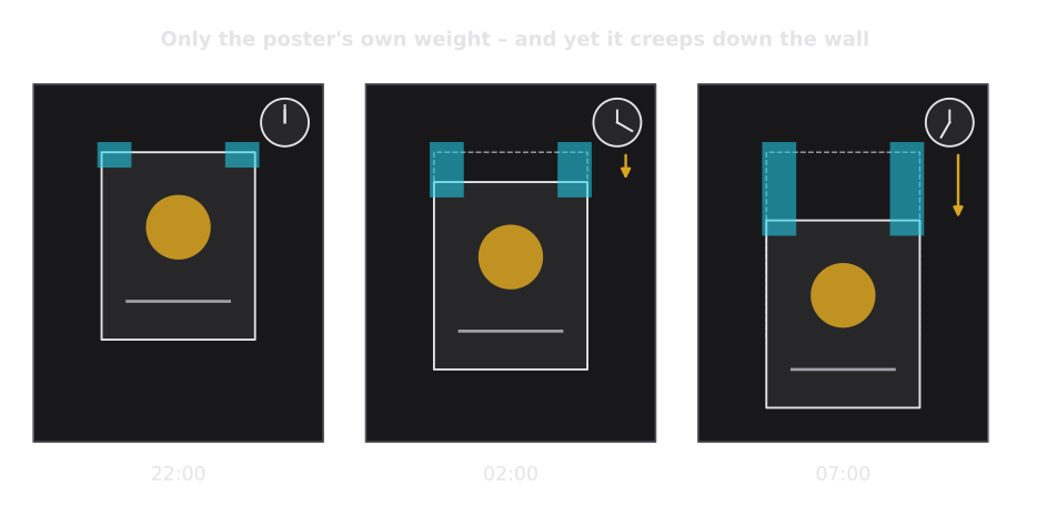
What to look for: the load never changes – it is always just the weight of the poster. The deformation still keeps growing with time. That is the signature of creep.

The Creep Test: Constant Stress, Growing Deformation

In the tests of Part 2 we set a speed and measured a force. A creep test works the other way round and is simpler to picture: we apply a constant shear stress $\tau_0$ and simply watch what the sample does.

The test has two phases:

1. Creep phase: at time $t = 0$, the rheometer suddenly applies the stress $\tau_0$ and holds it constant until time $t_1$. The deformation $\gamma(t)$ is recorded.
2. Recovery phase: at $t_1$ the stress is removed ($\tau = 0$), and we keep recording. Now we see which part of the deformation comes back.

Because the rheometer controls the stress, this is a test in controlled shear stress (CSS) mode. Modern rheometers with air bearings can apply stresses of well below 1 Pa and resolve deformations of a few millionths – ideal for watching a material creep.

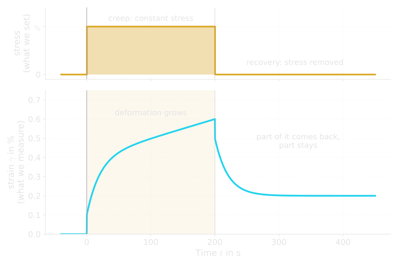
What to look for: the input (top) is a simple block. The output (bottom) is not: it jumps, bends, keeps rising, and after unloading it only partly returns. Every feature of this curve has a physical meaning – we decode them one by one below.

Creep Compliance: Softness Measured Over Time

If you pull twice as hard on a soft material, it deforms about twice as much. To compare tests at different stresses, we divide the deformation by the stress. The result is the creep compliance:

$J(t) = \frac{\gamma(t)}{\tau_0}$

In words: the creep compliance is the deformation per unit of stress. It tells you how soft a material is – and, unlike a single number, how this softness develops with time. Its unit is $1/\mathrm{Pa}$ ($\mathrm{Pa^{-1}}$). A large $J$ means soft; a small $J$ means stiff.

For an ideal spring (Part 3), the compliance is simply the inverse of the shear modulus: $J = 1/G$. A rubber with $G = 1$ MPa has $J = 10^{-6}\ \mathrm{Pa^{-1}}$; a soft adhesive with $G = 100$ kPa has $J = 10^{-5}\ \mathrm{Pa^{-1}}$. For viscoelastic materials $J$ grows with time – the material seems to get softer the longer you push.

Worked example. A tape adhesive is loaded with $\tau_0 = 100$ Pa. After 200 s, the rheometer reports a deformation of $\gamma = 0.006$ (that is 0.6 %). The creep compliance at this moment is $J(200\ \mathrm{s}) = 0.006 / 100\ \mathrm{Pa} = 6 \times 10^{-5}\ \mathrm{Pa^{-1}}$.

The Linearity Check

Dividing by the stress only makes sense if the deformation really is proportional to the stress. This is the case in the linear viscoelastic range – for small stresses, where the material’s inner structure is not changed by the test. The check is simple: run the creep test at two or three different stresses and plot $J(t)$. If the curves lie on top of each other, you are in the linear range.

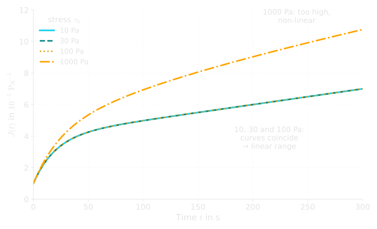
What to look for: three stresses, one curve – that is the proof of linearity. At 1000 Pa the structure of the material starts to give way, the compliance is larger, and the result would no longer be a material property but a property of this particular test.

Quick check: You measure $J(100\ \mathrm{s}) = 5 \times 10^{-5}\ \mathrm{Pa^{-1}}$ at 50 Pa and $J(100\ \mathrm{s}) = 8 \times 10^{-5}\ \mathrm{Pa^{-1}}$ at 500 Pa. Is 500 Pa inside the linear range? (No – the compliance depends on the stress. Stay at 50 Pa or below.)

Four Ways to Respond

Before we look at real materials, let us see how the ideal materials from the earlier parts respond to the same block of stress. The four answers look completely different – which makes the creep test a very good “fingerprint”.

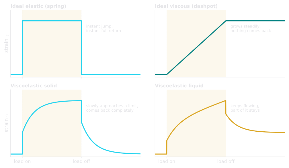
What to look for: the recovery phase separates the four cases most clearly. The spring gives back everything at once, the dashpot gives back nothing, and the viscoelastic materials give back something – with a delay.

Material	During creep	After unloading	Everyday example
Ideal elastic (spring)	Instant jump, then constant	Instant, complete recovery	Steel spring, rubber band
Ideal viscous (dashpot)	Straight-line increase	Nothing recovers	Honey, water
Viscoelastic solid	Slow approach to a final value	Complete, delayed recovery	Memory foam, crosslinked rubber
Viscoelastic liquid	Approaches a rising straight line	Partial recovery, permanent deformation	Silly Putty, polymer melts, most tape adhesives

Everyday example – chewing gum under your shoe: Step on a piece of chewing gum and lift your foot slowly. The gum stretches into a long thread (creep), and when it finally lets go, the thread snaps back partly – but a flattened, deformed piece stays on the pavement. Chewing gum is a viscoelastic liquid.

The Burgers Model: One Curve, Three Stories

In Part 4 we met two simple models: the Maxwell model (spring and dashpot in series, a viscoelastic liquid) and the Kelvin–Voigt model (spring and dashpot in parallel, a viscoelastic solid). Neither alone describes the curve of a real adhesive. But if we connect them one behind the other, we get the four-element Burgers model – and it reproduces the typical creep curve remarkably well.

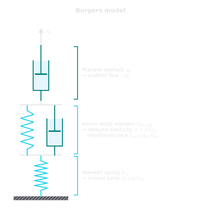
What to look for: each of the three parts has its own job. Cyan springs store energy and give it back; teal dashpots dissipate energy and never give it back.

Because the three parts are connected in series, they all carry the same stress $\tau_0$, and their deformations simply add up. Divided by $\tau_0$, this gives the creep compliance of the Burgers model:

$J(t) = J_0 + J_1\left(1 - e^{-t/\lambda_{ret}}\right) + \frac{t}{\eta_0}$

In words: the softness at time $t$ is the sum of three contributions:

• Instant elasticity $J_0 = 1/G_M$: the Maxwell spring stretches immediately when the load is applied. This is the vertical jump at $t = 0$.
• Delayed elasticity $J_1\left(1 - e^{-t/\lambda_{ret}}\right)$: the Kelvin–Voigt spring also wants to stretch, but its parallel dashpot slows it down. The deformation builds up gradually with the retardation time $\lambda_{ret} = \eta_K/G_K$. After one $\lambda_{ret}$, 63 % of $J_1$ is reached; after five, more than 99 %.
• Viscous flow $t/\eta_0$: the Maxwell dashpot flows steadily for as long as the stress acts. Its viscosity is the zero-shear viscosity $\eta_0$ – the viscosity of the material at rest, which we met as the low-shear plateau of the flow curve in Part 2.

In the language of Part 4: the first two parts are the “solid” memory of the material, the third part is its “liquid” side. A viscoelastic solid, like memory foam, simply lacks the third part ($\eta_0 \to \infty$).

Reading the Curve

Let us put in numbers for a typical general-purpose tape adhesive, which we call Tape B in this series: $J_0 = 1 \times 10^{-5}\ \mathrm{Pa^{-1}}$, $J_1 = 3 \times 10^{-5}\ \mathrm{Pa^{-1}}$, $\lambda_{ret} = 20$ s and $\eta_0 = 10^7$ Pa·s. We load it for $t_1 = 200$ s and then let it recover.

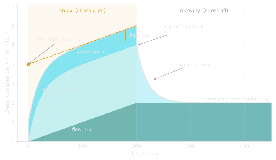
What to look for: the three colored bands are the three parts of the Burgers model. In recovery, the bright band (instant elasticity) disappears at once, the middle band (delayed elasticity) melts away within about a minute – and the bottom band (flow) stays forever.

Worked example – creep phase. At $t_1 = 200$ s, the delayed part is complete ($e^{-200/20} = e^{-10} \approx 0$):

$J(200\ \mathrm{s}) = 1 \times 10^{-5} + 3 \times 10^{-5} + \frac{200\ \mathrm{s}}{10^7\ \mathrm{Pa \cdot s}} = 6 \times 10^{-5}\ \mathrm{Pa^{-1}}$

With $\tau_0 = 100$ Pa, the deformation is $\gamma = J \cdot \tau_0 = 0.006$, i.e. 0.6 %. Of this, 0.1 % came instantly, 0.3 % with a delay, and 0.2 % is flow.

Behind the Burgers parameters are the element values: $G_M = 1/J_0 = 100$ kPa, $G_K = 1/J_1 \approx 33$ kPa and $\eta_K = \lambda_{ret} \cdot G_K \approx 6.7 \times 10^5$ Pa·s.

Creep Recovery: What Comes Back?

The recovery phase is the most revealing part of the test, because it separates what the material stored from what it lost. For the Burgers model, with $t' = t - t_1$ the time since unloading:

$\frac{\gamma(t')}{\tau_0} = J_1\left(1 - e^{-t_1/\lambda_{ret}}\right)e^{-t'/\lambda_{ret}} + \frac{t_1}{\eta_0}$

In words: the instant part $J_0$ has already jumped back at the moment of unloading and no longer appears. The delayed part fades away exponentially with the same retardation time $\lambda_{ret}$ with which it was built up. The flow part $t_1/\eta_0$ – everything the dashpot flowed during the creep phase – remains as permanent deformation.

Worked example – recovery phase. For Tape B:

• Immediately at unloading, the strain drops by $J_0 \tau_0 = 0.1$ % – from 0.6 % to 0.5 %.
• After another 60 s ($3\,\lambda_{ret}$), only 5 % of the delayed part is left: the strain is about 0.215 %.
• In the end, $t_1/\eta_0 = 2 \times 10^{-5}\ \mathrm{Pa^{-1}}$ remains – a permanent strain of 0.2 %, one third of the maximum.

The amount that came back is called the recovery compliance $J_R(t') = [\gamma(t_1) - \gamma(t_1 + t')]/\tau_0$. Here it ends at $4 \times 10^{-5}\ \mathrm{Pa^{-1}}$ – exactly the elastic parts $J_0 + J_1$.

Everyday example – the memory-foam mattress: When you get up from a memory-foam mattress, the imprint of your body is visible for a few seconds and then fades – that is delayed recovery. Because memory foam is a crosslinked (viscoelastic) solid, it eventually recovers completely. An old, worn pillow of soft foam or feathers keeps a dent – its “flow part” has become permanent.

Finding the Zero-Shear Viscosity – Without Rushing

One of the most important uses of a creep test is to measure the zero-shear viscosity $\eta_0$: the viscosity at rest, at shear rates far too low for a rotational test. It is also a key number for the holding power of adhesives.

The trick is that at long times, every viscoelastic liquid – whatever its inner structure – ends up in a steady state. The elastic parts are “used up”, and only flow continues:

$J(t) \approx J_e^0 + \frac{t}{\eta_0}$

In words: at long times the creep curve turns into a straight line. Its slope is $1/\eta_0$, and extrapolated back to $t = 0$ it hits the steady-state compliance $J_e^0$, the total elastic softness of the material. For the Burgers model, $J_e^0 = J_0 + J_1$. Nice detail: this recipe works without any model – it applies to real materials with many retardation times as well.

Worked example. From the goldenrod line in the figure above: between 120 s and 180 s, $J$ rises from $5.2$ to $5.8 \times 10^{-5}\ \mathrm{Pa^{-1}}$. The slope is $0.6 \times 10^{-5}\ \mathrm{Pa^{-1}} / 60\ \mathrm{s} = 10^{-7}\ \mathrm{Pa^{-1}\,s^{-1}}$, so $\eta_0 = 1/\text{slope} = 10^7$ Pa·s. The intercept gives $J_e^0 = 4 \times 10^{-5}\ \mathrm{Pa^{-1}}$.

The Classic Mistake: Evaluating Too Early

The steady state takes time to arrive. As long as the delayed elasticity is still active, the curve rises faster than the pure flow part. If you draw the straight line too early, you measure too steep a slope – and therefore a too low zero-shear viscosity.

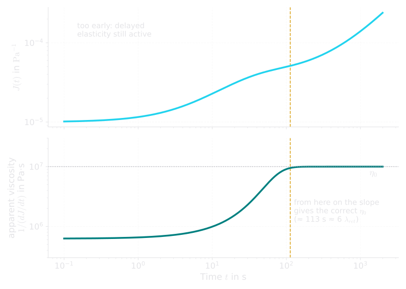
What to look for: the lower panel shows the viscosity you would calculate from the local slope. Read too early, it can be more than ten times too small. Only after roughly six retardation times does it reach its true value.

A practical rule: the creep phase must last several times the longest retardation time of the material. Two checks help in the lab:

• The local slope $dJ/dt$ must no longer change – the apparent viscosity $1/(dJ/dt)$ must have reached a plateau, as in the lower panel.
• On a log–log plot, the curve bends upward towards a slope of 1 (a straight proportional rise, $J \propto t$). Once it gets close, flow clearly dominates the elastic parts.

A useful by-product: the product of the two steady-state numbers is a time,

$\lambda_0 = \eta_0 \cdot J_e^0$

In words: the mean relaxation time tells how long the material “remembers” a deformation on average. For Tape B, $\lambda_0 = 10^7\ \mathrm{Pa \cdot s} \times 4 \times 10^{-5}\ \mathrm{Pa^{-1}} = 400$ s. We will meet this time again in Parts 6 and 7.

In the lab – good creep practice:

• Stress: choose $\tau_0$ inside the linear range; check it with a second stress (the $J(t)$ curves must coincide).
• Duration: the creep phase should last several times the longest retardation time – for polymer melts and adhesives often many minutes to hours. Allow a recovery phase of similar length.
• Creep ringing: right after the stress step, the curve may oscillate for a fraction of a second. This is not the material misbehaving: the inertia of the rotating measuring system swings against the elastic sample like a mass on a spring. Ignore the first moments or use them deliberately – the frequency of the ringing contains information about the elastic modulus.
• Temperature: creep depends strongly on temperature; a drift of 1 K during a long test changes $\eta_0$ noticeably. Let the sample equilibrate and keep the temperature constant.
• Sample loading: loading squeezes the sample and leaves stresses behind. Wait until the normal force has relaxed before you start.

Try it at home – tape creep: Take three different tapes (for example masking tape, office tape and a strong packaging tape). Stick a strip of each to the edge of a table so that exactly 2 cm × 2 cm are bonded and the rest hangs down. Attach the same weight to each, for example a full 0.5 L water bottle (use a lighter one if a tape lets go at once), and mark the lower edge of the bond with a pencil. Mark it again every hour. The distance between the marks over time is a real creep curve – and half a kilogram on 4 cm² gives about 12 kPa, close to the stress of the standard industrial test described below.

Three Tapes, Three Creep Curves

Let us now compare the three model adhesives of this series. Tape A is a removable label adhesive – soft and easy to peel off. Tape B is the general-purpose tape from our worked example. Tape C is a high-shear mounting tape that has to hold heavy loads for years.

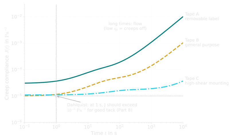
What to look for: at short times (left) all three tapes are soft enough to stick. At long times (right) they separate by orders of magnitude: Tape A flows away, Tape C hardly moves.

The comparison shows the classic dilemma of adhesive design:

• Short times – bonding. To wet a surface when you press it on, an adhesive must be soft within about a second. As early as the 1960s, Carl Dahlquist found that tapes are only tacky when their creep compliance at 1 s exceeds about $10^{-5}\ \mathrm{Pa^{-1}}$ – in other words, when their modulus is below about 100 kPa. All three tapes pass; Tape C only just. We come back to this Dahlquist criterion in Part 8.
• Long times – holding. To carry a load for hours or years, the adhesive must hardly flow: its zero-shear viscosity must be high. Here Tape C ($\eta_0 = 5 \times 10^8$ Pa·s) beats Tape A ($\eta_0 = 10^6$ Pa·s) by a factor of 500.

Holding Power: The Creep Test of the Adhesives Industry

The adhesives industry has its own, very practical creep test: the static shear test, often called the holding-power test (standardized, for example, as PSTC-107, FINAT FTM 8 and ASTM D3654). A strip of tape is bonded to a vertical steel plate over a defined area – typically 25 mm × 25 mm – and a weight, often 1 kg, hangs from its free end. A timer records how long it takes until the tape slides off.

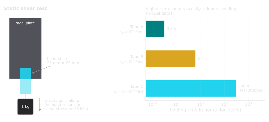
What to look for: the weight is a constant load – exactly like the constant stress of a rheometer creep test. The ranking of the holding times follows the ranking of the zero-shear viscosities.

Worked example. The weight pulls with $F = m \cdot g = 1\ \mathrm{kg} \times 9.81\ \mathrm{m/s^2} \approx 9.8$ N. Spread over the bonded area $A = 0.025\ \mathrm{m} \times 0.025\ \mathrm{m} = 6.25 \times 10^{-4}\ \mathrm{m^2}$, this is a shear stress of

$\tau_0 = \frac{F}{A} = \frac{9.8\ \mathrm{N}}{6.25 \times 10^{-4}\ \mathrm{m^2}} \approx 16\ \mathrm{kPa}$

That is more than a hundred times the stress we used in the rheometer. The static shear test is therefore a creep test far outside the linear range – a test “to failure”. But the underlying physics is the same: a tape with a high zero-shear viscosity and a small long-time compliance creeps slowly and holds for a long time.

Common pitfall – “high holding power” is not a free lunch: Making an adhesive hold longer usually means making it stiffer and more viscous – which also makes it less tacky and harder to press on. Tape C holds for weeks but needs firm pressure to bond; Tape A sticks at a touch but lets go under a steady load. Finding the balance is the art of adhesive formulation.

Why It Matters for Adhesives

For a pressure-sensitive adhesive, the creep curve is almost a complete résumé:

• The short-time compliance (around 1 s) tells whether the adhesive is soft enough to wet a surface quickly – tack.
• The zero-shear viscosity $\eta_0$ tells how fast the adhesive flows under a permanent load – holding power, the tendency of labels to “swim” on a curved bottle, or of a tape roll to ooze at its edges.
• The recovery tells how much of a deformation is stored elastically. A mounting tape that springs back after a load has been removed keeps its shape; one that has flowed permanently does not.

The poster on the wall is therefore a small creep test that you run every night. A poster tape with a high $\eta_0$ keeps the poster in place; one that flows too easily lets it slide – or, as the adhesive flows into the wallpaper, leaves a mark when you remove it.

Key Takeaways

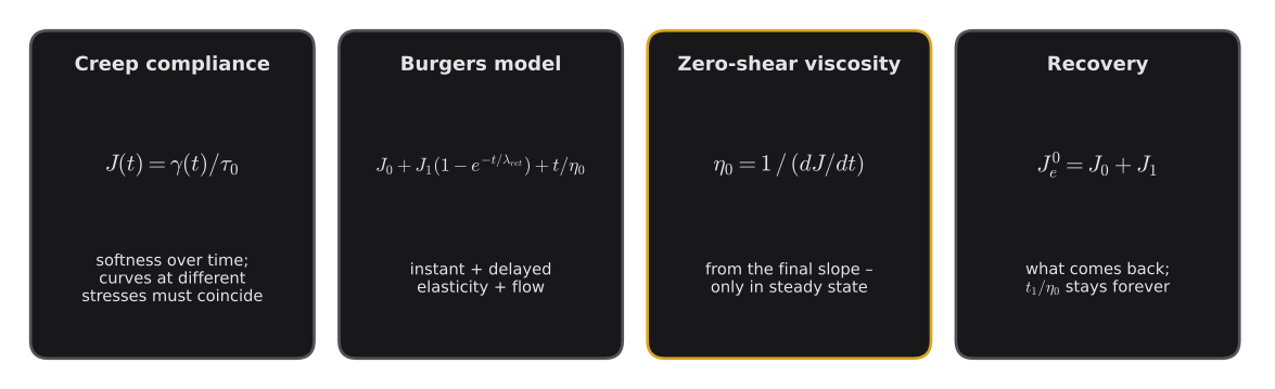
• In a creep test, a constant stress is applied and the growing deformation is recorded; in the recovery phase, the stress is removed and we see what comes back.
• The creep compliance $J(t) = \gamma(t)/\tau_0$ measures softness over time. Curves at different stresses that lie on top of each other prove that the test is in the linear range.
• The Burgers model splits the creep curve into instant elasticity ($J_0$), delayed elasticity ($J_1$, $\lambda_{ret}$) and flow ($t/\eta_0$).
• In recovery, the elastic parts come back – instantly and with a delay – while the flowed part $t_1/\eta_0$ remains as permanent deformation.
• The zero-shear viscosity $\eta_0$ comes from the final slope, the steady-state compliance $J_e^0$ from the intercept – but only once the steady state is reached. Evaluating too early gives a too low $\eta_0$.
• For tapes, the static shear test is the industrial version of a creep test: a high $\eta_0$ means a long holding time.

Key Terms

Term	Meaning in plain language	Symbol, unit
Creep	Deformation that keeps growing under constant load	–
Creep recovery	Return of deformation after the load is removed	–
Creep compliance	Deformation per unit of stress – “softness over time”	$J(t)$, $\mathrm{Pa^{-1}}$
Instant compliance	The immediate elastic jump	$J_0$, $\mathrm{Pa^{-1}}$
Delayed compliance	The elastic part that builds up with a delay	$J_1$, $\mathrm{Pa^{-1}}$
Retardation time	How long the delayed elasticity takes	$\lambda_{ret}$, s
Zero-shear viscosity	Viscosity at rest, from the final slope	$\eta_0$, Pa·s
Steady-state compliance	Total elastic softness, from the intercept	$J_e^0$, $\mathrm{Pa^{-1}}$
Recovery compliance	How much of the deformation came back	$J_R$, $\mathrm{Pa^{-1}}$
Mean relaxation time	Average “memory time” of the material	$\lambda_0 = \eta_0 J_e^0$, s
Burgers model	Maxwell and Kelvin–Voigt model in series	–
Creep ringing	Short oscillation after the stress step, caused by instrument inertia	–
Static shear test	Holding-power test: a weight hanging on a bonded tape	holding time, h

Coming Up Next

A rubber band wrapped tightly around a bundle of old letters grips them firmly today. Find the bundle again years later: the band is still stretched to the same length – but it hardly holds anything. Its inner tension has faded away. In Part 6 we turn the creep test around: instead of a constant load, we apply a constant deformation and watch the stress relax – and discover why real materials need not one, but a whole orchestra of relaxation times.

References

1. Mezger, T. G.: The Rheology Handbook, 5th ed., Vincentz Network, Hanover 2020.
2. Macosko, C. W.: Rheology: Principles, Measurements, and Applications, Wiley-VCH, New York 1994.
3. Ferry, J. D.: Viscoelastic Properties of Polymers, 3rd ed., Wiley, New York 1980.
4. Findley, W. N.; Lai, J. S.; Onaran, K.: Creep and Relaxation of Nonlinear Viscoelastic Materials, North-Holland, Amsterdam 1976.
5. Dahlquist, C. A.: Tack, in: Adhesion Fundamentals and Practice, Maclaren, London 1969, pp. 143–151.
6. Pressure Sensitive Tape Council: PSTC-107 – Shear Adhesion of Pressure Sensitive Tape, Test Methods for Pressure Sensitive Adhesive Tapes, Oak Brook, IL.
7. FINAT: FINAT Test Method No. 8 – Resistance to Shear from a Standard Surface, FINAT Technical Handbook, The Hague.