10 Interactive Rheometer: Watch a Flow Curve Being Measured

In Part 2 we met the rotational rheometer as a drawing and looked at finished curves. But what actually happens during a measurement? What does the instrument set, what does it measure, and how does a curve grow out of it, point by point?

This part is different from the others: instead of reading, you can run the measurement yourself. Below is a virtual rheometer with a bob-and-cup geometry, filled with water at 20 °C. Press start, watch the bob begin to turn, see the torque tick up – and follow the flow curve and the viscosity curve as they build up live.

What to look for: the bob turns faster with every point, the torque rises in step – and the viscosity stays at the same value from the first point to the last. That is what “Newtonian” looks like in a real measurement.

How to use it:

• ▶ Start measurement runs the test: 21 shear rates from 1 to 100 s⁻¹. Pause and Reset do what they say.
• Speed compresses the measuring time. A real test of this kind takes about two minutes; the display always shows the real test time.
• Sample lets you swap water for a silicone oil or glycerol.
• Expert mode extends the test to 1000 s⁻¹. Try it with water – and read the section on Taylor vortices below.
• If your device is set to reduce motion, the rotation is not animated and you measure point by point with a button.

All values are model data, calculated from the equations explained below.

What You Are Looking At

The virtual instrument uses a concentric cylinder geometry, often called “bob and cup”: a cylinder (the bob) hangs from the measuring head into a cup filled with the sample. The bob rotates; the cup stands still and is temperature-controlled. The liquid is sheared in the narrow ring-shaped gap between them.

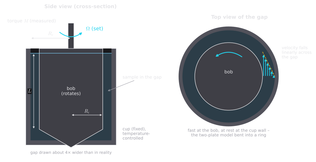
What to look for: the gap is only about 1 mm wide. Across it, the liquid speed falls from the speed of the bob surface to zero at the cup wall – exactly like the liquid between the two plates of Part 1, just bent into a ring.

The tracer particles in the top view of the interactive show the same thing: particles close to the bob race around, particles close to the cup wall hardly move.

Our virtual instrument uses a standard geometry described in ISO 3219, often called CC27:

Quantity	Value
Bob radius $R_i$	13.33 mm
Cup radius $R_e$	14.46 mm (ratio $R_e/R_i$ = 1.0847)
Gap	1.13 mm
Bob length $L$	40 mm
Sample volume	about 19 mL

The ratio of the two radii is fixed by the standard. It keeps the gap so narrow that the shear rate is almost the same everywhere in it – it varies by only about ±8 % around the value in the middle of the gap.

What Happens When You Press Start

The test runs in controlled shear rate mode (CSR, Part 2): the rheometer sets a speed, waits until the flow is steady and measures the torque it needs to keep the bob turning. Then it moves on to the next speed.

The instrument never measures shear rate or shear stress directly. It knows only two raw quantities – the rotational speed $n$ and the torque $M$ – and converts them with constants that depend only on the geometry:

$\dot{\gamma} = 1.291 \cdot n, \qquad \tau = \frac{0.0446 \cdot M}{R_i^3}, \qquad \eta = \frac{\tau}{\dot{\gamma}}$

In words: the shear rate is proportional to the rotational speed (with $n$ in revolutions per minute), and the shear stress is proportional to the torque divided by the cube of the bob radius. Their ratio is the viscosity. The numbers 1.291 and 0.0446 hold for every ISO standard cylinder; they come from the geometry of the gap and refer to its middle.

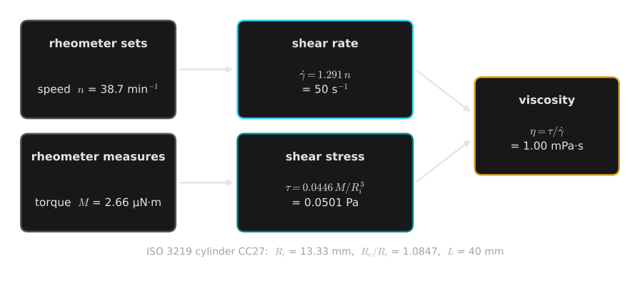
What to look for: two raw numbers in, three rheological numbers out. Everything a rotational rheometer reports is calculated this way.

Worked example. At point 18 of the test, the rheometer sets $\dot{\gamma} = 50\ \mathrm{s^{-1}}$. The bob therefore turns at $n = 50 / 1.291 = 38.7$ revolutions per minute – less than one turn per second. Water resists with a torque of only $M = 2.66\ \mathrm{\mu N \cdot m}$. That gives

$\tau = \frac{0.0446 \times 2.66\times10^{-6}\ \mathrm{N\,m}}{(0.01333\ \mathrm{m})^3} = 0.0501\ \mathrm{Pa}, \qquad \eta = \frac{0.0501\ \mathrm{Pa}}{50\ \mathrm{s^{-1}}} = 1.00\ \mathrm{mPa\cdot s}$

A torque of 2.66 µN·m is tiny: about the torque of a single grain of rice (0.03 g) resting on the end of a 1 cm lever. Rheometers can measure it only because the bob hangs in an almost frictionless air bearing.

Why Every Point Takes a Few Seconds

Watch the display while a point is being measured: when the speed jumps to the next value, the torque does not jump at once – it approaches its new value within a moment. The rheometer first waits until the flow is steady (in our model 2 s) and then averages the torque over a measuring window (4 s). Only then is the point drawn. With 21 points, the whole test takes a little over two minutes.

For water, steady flow is reached almost instantly. For structured samples – ketchup, paint, a polymer solution – the waiting time matters much more, because their structure needs time to adjust to each new shear rate (Part 2).

Reading the Two Curves

When the test is finished, two curves appear:

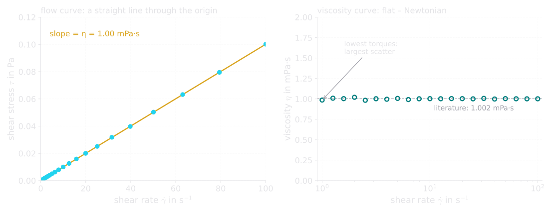
What to look for: a straight line through the origin on the left, a horizontal line on the right. Both say the same thing: the viscosity of water does not depend on how fast it is sheared.

• The flow curve ($\tau$ over $\dot{\gamma}$, linear axes) is a straight line through the origin. Its slope is the viscosity: $\tau = \eta\,\dot{\gamma}$.
• The viscosity curve ($\eta$ over $\dot{\gamma}$, usually with a logarithmic shear-rate axis) is a horizontal line at 1.00 mPa·s – the literature value for water at 20 °C is 1.002 mPa·s.

Water is a Newtonian liquid – the simplest case of all. Compare this with the curves of Part 2, where ketchup and paint gave curved flow curves and falling viscosity curves:

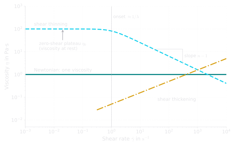
What to look for: water produces the flat line. Everything that is not flat is a sign of structure inside the material.

Try it in the interactive: Choose glycerol as the sample and run the test again. The torque is now about 1,400 times higher – glycerol is 1,400 times more viscous than water – but the curves have exactly the same shape: glycerol is Newtonian too. Viscosity tells you how thick a liquid is; the shape of the curves tells you how it behaves.

Why the First Points Wobble

Look closely at the first few points of the viscosity curve: they scatter a little more than the rest. At 1 s⁻¹, water produces a torque of only 53 nN·m – about fifty billionths of a newton meter. The electronic noise and the residual friction of the instrument, a few nanonewton meters, then amount to several percent of the signal.

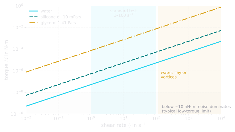
What to look for: every liquid has a “measuring window” – above the noise at low shear rates and below disturbances at high shear rates. For water, this window is surprisingly narrow.

This is a general rule: thin liquids at low shear rates are the hardest measurements in rheology. Larger geometries – for example a double-gap cylinder with two shearing surfaces – give more torque and thus cleaner data.

Expert Mode: When Water Seems to Get Thicker

Now switch on expert mode and run the test with water up to 1000 s⁻¹. Up to about 116 s⁻¹, nothing changes. Beyond that point, the measured viscosity starts to rise – at 1000 s⁻¹ water seems three times thicker than it is. Has the water changed? No. The flow has changed.

When the bob rotates fast, the liquid near it is flung outward by centrifugal force, while the liquid near the fixed cup wall is slow. Above a critical speed, this arrangement becomes unstable, and the liquid rolls up into stacked, ring-shaped Taylor vortices – named after G. I. Taylor, who described them in 1923. These vortices carry momentum across the gap and dissipate extra energy. The rheometer measures a higher torque and – since it assumes smooth, layered flow – reports a higher viscosity.

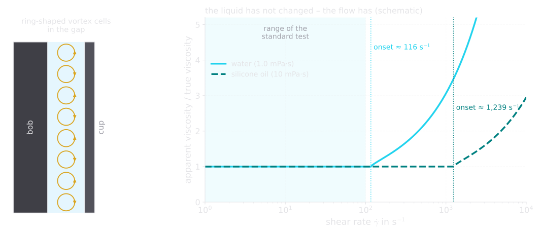
What to look for: the apparent viscosity rises although the liquid has not changed. A ten times more viscous liquid stays stable up to a ten times higher shear rate.

The onset can be calculated from the Taylor number. For a narrow-gap cylinder with a rotating bob, the critical angular velocity (DIN 53019-3, Mezger) is

$\omega_c = \frac{41.2\,\eta}{\rho\,R_i^2\,(R_e/R_i - 1)^{3/2}}$

In words: the higher the viscosity $\eta$, the more stable the flow; the higher the density $\rho$ and the larger the bob, the earlier the vortices appear. A thin, heavy liquid in a large bob is the worst case.

Worked example. For water ($\eta = 1.002$ mPa·s, $\rho = 998$ kg/m³) in CC27:

$\omega_c = \frac{41.2 \times 1.002\times10^{-3}}{998 \times (0.01333)^2 \times (0.0847)^{3/2}} \approx 9.4\ \mathrm{rad/s} \quad\Rightarrow\quad \dot{\gamma}_c = 12.33\,\omega_c \approx 116\ \mathrm{s^{-1}}$

Above about 116 s⁻¹, water can no longer be measured correctly with this geometry. For the 10 mPa·s silicone oil, the limit rises tenfold to about 1,240 s⁻¹; for glycerol, it lies far beyond any practical speed.

Common pitfall – “my water is shear-thickening”: Every year, somebody measures water, a solvent or a thin beverage in a cylinder geometry up to high shear rates and “discovers” shear thickening. It is almost always Taylor vortices. Check the critical shear rate before you interpret a rising viscosity of a thin liquid. Rheometers with a rotating cup and a fixed bob (Couette principle) do not show Taylor vortices at all – the centrifugal force then pushes the fast liquid outward against the stable, slow liquid near the bob – but at still higher speeds, ordinary turbulence sets a limit for them, too.

In the interactive, the vortices are drawn schematically, and the rise of the apparent viscosity follows a simple illustrative model – the real rise depends on the geometry and on the liquid.

In the lab – measuring thin liquids in a cylinder:

• Fill level: fill to the mark. Too little or too much liquid changes the effective length of the bob and therefore the torque.
• Bubbles: air bubbles in the gap reduce the torque. Fill slowly and lower the bob gently.
• Temperature: water loses about 2–3 % of its viscosity per kelvin. Wait until the sample has reached the set temperature, typically a few minutes.
• Evaporation: at elevated temperatures, use a cover (solvent trap); a drop in fill level shows up as a slowly falling viscosity.
• Low torque: check that the lowest points are well above the minimum torque of your instrument, or choose a larger or double-gap geometry.
• High shear rate: calculate the Taylor limit before you start and stay below it.

Why It Matters for Adhesives

Many adhesives begin their life as a liquid: acrylic pressure-sensitive adhesives are often produced as water-based dispersions or as solutions in organic solvents, and they are coated onto the backing as a thin liquid film. Their viscosity decides whether the coating runs smoothly, forms streaks or drips – and it is measured exactly as shown here, usually in a bob-and-cup geometry. Unlike water, these liquids are rarely Newtonian: dispersions are typically shear-thinning, which is why the whole flow curve, not a single value, is measured.

Once the adhesive has dried into a soft, sticky film, the bob and cup are no longer suitable. The film is placed between two plates and probed gently back and forth – the oscillation test of Part 7. That is what Part 11 lets you watch.

Key Takeaways

• A rotational rheometer sets the speed $n$ and measures the torque $M$; shear rate, shear stress and viscosity are calculated from them with geometry constants.
• In a bob-and-cup geometry, the liquid is sheared in a narrow ring-shaped gap – the two-plate model bent into a ring.
• Each point needs a short settling time and a measuring window; a test with 21 points takes about two minutes.
• Water is Newtonian: a straight flow curve through the origin and a flat viscosity curve at 1.00 mPa·s (20 °C).
• Thin liquids produce tiny torques – the first points scatter most. Every liquid and geometry has a measuring window.
• Above a critical shear rate – about 116 s⁻¹ for water in CC27 – Taylor vortices make the viscosity seem to rise. That is a measuring artifact, not shear thickening.

Key Terms

Term	Meaning in plain language	Symbol, unit
Bob and cup	Concentric cylinder geometry: a rotating cylinder inside a cup	–
Searle principle	The inner cylinder (bob) rotates, the cup is fixed	–
Couette principle	The cup rotates, the bob is fixed	–
Rotational speed	Revolutions of the bob per minute	$n$, min⁻¹
Torque	Twisting force needed to keep the bob turning	$M$, N·m
CSR	Controlled shear rate: the rheometer sets the speed	–
Measuring window	Time over which the torque is averaged for one point	s
Newtonian liquid	Viscosity independent of shear rate	–
Air bearing	Almost frictionless bearing of the measuring shaft	–
Taylor vortices	Ring-shaped vortices in the gap at high bob speeds	–
Critical shear rate	Onset of Taylor vortices	$\dot{\gamma}_c$, s⁻¹

Coming Up Next

In Part 11 we swap the water for a disk of acrylic adhesive and the rotating bob for two parallel plates. The upper plate twists back and forth – first fast, then slower and slower – and you can watch the strain and the stress swing out of step while $G'$, $G''$ and $\tan\delta$ build up into a frequency sweep: the measurement behind the Chang window.

References

1. Mezger, T. G.: The Rheology Handbook, 5th ed., Vincentz Network, Hanover 2020 (chapter 10.2: concentric cylinder measuring systems, Taylor vortices).
2. ISO 3219-2: Rheology – Part 2: General principles of rotational and oscillatory rheometry, International Organization for Standardization, Geneva.
3. DIN 53019-1: Viscometry – Measurement of viscosities and flow curves by means of rotational viscometers – Part 1: Principles and measuring geometry, Beuth, Berlin.
4. DIN 53019-3: Viscometry – Measurement of viscosities and flow curves by means of rotational viscometers – Part 3: Measurement uncertainties, Beuth, Berlin.
5. Taylor, G. I.: Stability of a viscous liquid contained between two rotating cylinders, Philosophical Transactions of the Royal Society A 223 (1923) 289–343.
6. Huber, M. L. et al.: New international formulation for the viscosity of H₂O, Journal of Physical and Chemical Reference Data 38 (2009) 101–125.
7. Macosko, C. W.: Rheology: Principles, Measurements, and Applications, Wiley-VCH, New York 1994.