11 Interactive Rheometer: Watch a Frequency Sweep of an Adhesive

In Part 7 we learned what an oscillation test is: the rheometer twists a sample gently back and forth and compares the stress with the strain. In Part 8 we used the result – a frequency sweep – to place adhesives on Chang’s map. But what does it look like while the test is running? How do two swinging sine waves turn into $G'$, $G''$ and $\tan\delta$? And why does a single sweep keep a rheometer busy for more than an hour?

In this second interactive part, you run the test yourself. A disk of our general-purpose acrylic adhesive, Tape B, sits between two parallel plates at 23 °C. Press start and watch the upper plate twist – fast at first, then slower and slower – while the frequency sweep builds up point by point.

What to look for: the stress wave always runs slightly ahead of the strain wave – that head start is the phase angle δ. Watch how it changes as the frequency drops, and how each point appears in the sweep plot at the bottom.

How to use it:

• ▶ Start sweep runs the test: 16 frequencies from 100 down to 0.1 rad/s. Pause and Reset do what they say.
• Adhesive switches between the three model tapes of this series: Tape A (removable label), Tape B (general purpose) and Tape C (mounting tape).
• Display sets how fast the time lapse runs.
• Long version to 0.01 rad/s extends the sweep by one decade – and at the end draws your own Chang window from the measured values.
• If your device is set to reduce motion, the oscillation is not animated and you measure point by point with a button.

All values are model data, based on the relaxation spectra of the three tapes that we built up in Parts 5 to 8.

What You Are Looking At

For a soft solid like an adhesive film, the bob and cup of Part 10 are unsuitable – you cannot pour a sticky film into a cup. Instead, a disk of adhesive is placed between two flat, round plates. The lower plate is fixed and temperature-controlled; the upper plate, 25 mm in diameter (a “PP25” geometry), is lowered onto the sample and then twisted back and forth.

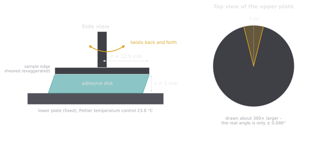
What to look for: the sample is sheared exactly like the deck of cards in Part 1 – the top slides relative to the bottom – but only by a tiny amount, and alternately in both directions.

The test conditions of our virtual measurement:

Quantity	Value
Geometry	Parallel plates PP25 ($R$ = 12.5 mm), gap $h$ = 1.0 mm
Sample	Tape B adhesive, laminated from several layers to 1 mm, punched to 25 mm
Temperature	23.0 °C
Mode	Controlled strain (CSD), amplitude $\gamma_0$ = 1 % – inside the linear range
Frequencies	100 → 0.1 rad/s, 5 points per decade (long version: down to 0.01 rad/s)

Worked example – how far does the plate turn? In a parallel-plate geometry, the strain at the rim is $\gamma = \varphi R / h$. For a strain amplitude of 1 %, the plate turns by

$\varphi_0 = \frac{\gamma_0\,h}{R} = \frac{0.01 \times 1\ \mathrm{mm}}{12.5\ \mathrm{mm}} = 8\times10^{-4}\ \mathrm{rad} \approx 0.046°$

The rim of the plate moves by $R\,\varphi_0 = 12.5\ \mathrm{mm} \times 8\times10^{-4} = 10\ \mathrm{\mu m}$ – about a seventh of the width of a human hair. That is why the animation shows the angle about 300 times larger than in reality.

The rheometer records the torque $M$ needed for this motion and converts it into the shear stress at the rim of the plate, $\tau_R = 2M/(\pi R^3)$. For Tape B, the torque amplitude is about 8 mN·m at 100 rad/s and about 1.3 mN·m at 0.1 rad/s – easy to measure, unlike the tiny torques of water in Part 10.

The Two Sine Waves

The two traces in the “live signals” panel are the heart of the test. The rheometer imposes the strain (cyan) as a smooth sine wave; the stress (teal, dashed) answers with the same frequency – but shifted in time by the phase angle $\delta$. On the right, the same two signals are plotted against each other: the tilted ellipse is the Lissajous loop from Part 7, and its area is the energy lost in each cycle.

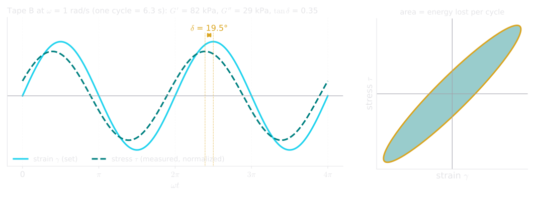
What to look for: a small phase shift and a narrow loop mean a mostly elastic material. A liquid would show a shift close to 90° and a nearly round loop.

From the two waves, the rheometer calculates everything else (Part 7):

$|G^*| = \frac{\tau_0}{\gamma_0}, \qquad G' = |G^*|\cos\delta, \qquad G'' = |G^*|\sin\delta, \qquad \tan\delta = \frac{G''}{G'}$

In words: the ratio of the two amplitudes gives the total stiffness; the phase angle splits it into a stored, elastic part $G'$ and a lost, viscous part $G''$.

Worked example. At $\omega$ = 1 rad/s, the rheometer measures a stress amplitude of $\tau_0$ = 874 Pa at $\gamma_0$ = 1 % and a phase angle of 19.5°:

• $|G^*| = 874\ \mathrm{Pa} / 0.01 = 87.4$ kPa
• $G' = 87.4 \times \cos 19.5° \approx 82$ kPa
• $G'' = 87.4 \times \sin 19.5° \approx 29$ kPa
• $\tan\delta = 29/82 \approx 0.35$ – clearly solid-like at this time scale.

Try it in the interactive: Pause the sweep at the start (100 rad/s) and look at the phase shift and the width of the loop. Then continue and pause again around 2 rad/s. The loop has become narrower – at this time scale, Tape B is at its most elastic ($\tan\delta \approx 0.30$). At the lowest frequencies, it opens up again.

The Curve Builds Up

Every few seconds, a new point appears in the sweep plot – from right to left, because the test runs from fast to slow. There are two practical reasons for this order. The fast points take only seconds, so a first overview is available immediately. And if the sample changes during the test – it dries, relaxes or loses contact – the damage shows up only in the last, slowest points.

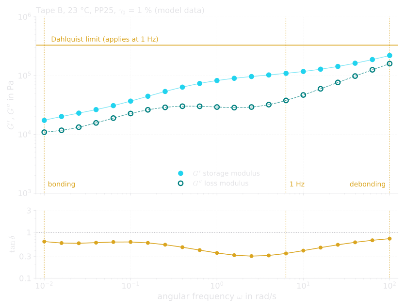
What to look for: Tape B is stiffer and more dissipative when deformed fast (right) and softer when deformed slowly (left) – the time dependence that makes it a good adhesive.

Reading the curves from fast to slow:

• At 100 rad/s (peeling): $G'$ and $G''$ are both high and close together, $\tan\delta \approx 0.73$. The adhesive is starting to enter its glass transition: it resists strongly and dissipates a lot of energy – the source of peel strength (Part 9).
• Around 1 to 3 rad/s (tack): the adhesive is at its most elastic, $\tan\delta \approx 0.3$. At 1 Hz, $G' \approx 110$ kPa – well below the Dahlquist limit of 330 kPa: Tape B is soft enough to grab on contact.
• At 0.01 rad/s (bonding): $G'$ has fallen to about 17 kPa and $\tan\delta$ has risen to about 0.6: the adhesive is soft and partly liquid-like, so it can flow into the roughness of a surface. But $G'$ stays above $G''$: it still does not flow away under a load – good holding power.

Why So Slow?

Watch the “real time” counter in the display: the first ten points take less than a minute in total, but the last few take several minutes each. Every point needs a few full oscillation cycles, and one cycle at 0.1 rad/s lasts 63 s – at 0.01 rad/s it lasts more than ten minutes.

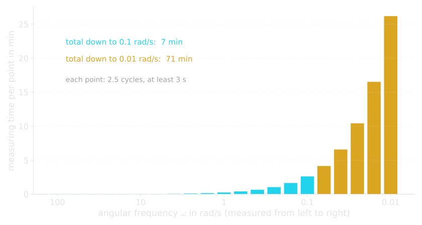
What to look for: the last decade of frequency costs almost ten times more time than all the others together.

This is the practical reason for time–temperature superposition (Part 8): instead of waiting an hour for 0.01 rad/s, the same information can be obtained by measuring at a higher temperature, where the adhesive “lives” faster, and shifting the curve. Our virtual sweep at a single temperature shows what TTS saves.

From Sweep to Chang Window

Tick “Long version” and run the sweep again. At the end, the interactive reads the four values at 0.01 and 100 rad/s and draws your own Chang window – the rectangle from Part 8 that places the adhesive on the map of pressure-sensitive adhesives. For Tape B, it lands in the central, general-purpose region.

Now try the other two tapes:

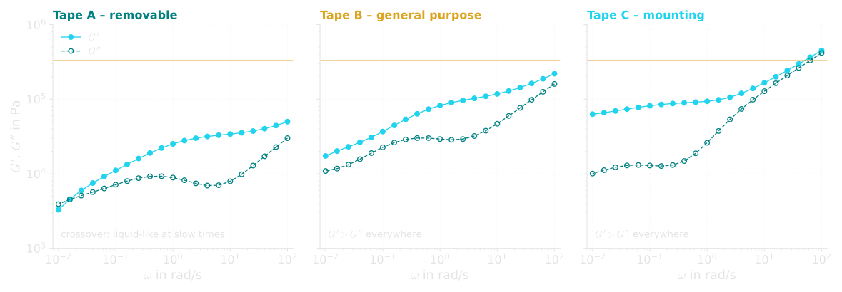
What to look for: three adhesives, three fingerprints. The differences at 0.01 and 100 rad/s are exactly what the Chang window condenses into a rectangle.

• Tape A is soft at every frequency, and at the slowest ones $G''$ overtakes $G'$: it wets surfaces easily and comes off cleanly – but it creeps under a permanent load.
• Tape C keeps a high, almost flat $G'$ at slow time scales – high cohesion and holding power – and becomes very stiff and dissipative at peel rates. Its window lies higher and further to the right on the Chang map.

In the lab – a good frequency sweep of an adhesive:

• Sample: laminate several layers of the adhesive film, free of bubbles, to about 1 mm, and punch a disk of the plate diameter. Trapped air makes the results too soft.
• Contact: lower the plate until it makes full contact, then keep a small, constant normal force during the test, so that the plate does not lose contact as the adhesive relaxes.
• Amplitude sweep first: check at the highest frequency and the lowest temperature of the test that the chosen strain lies inside the linear viscoelastic range (Part 7).
• Temperature: let the sample equilibrate for several minutes; near the glass transition, a single kelvin changes the moduli noticeably.
• Geometry: for stiff samples (cold temperatures) use smaller plates (e.g. 8 mm), for soft samples (warm temperatures) larger ones, so that the torque stays within the instrument’s range.

Why It Matters for Adhesives

The frequency sweep you just watched is the single most informative rheological test for a pressure-sensitive adhesive. From one curve you can read the softness for bonding, the tack at 1 Hz, the dissipation that drives peel strength and the cohesion that decides holding power – and with the four corner values, the Chang window. With features such as the loss integral, it also feeds the machine-learning model of Part 9.

Watching it being measured shows the other side of the coin: the numbers come from tiny motions of a few micrometers, from careful sample preparation, and from patience at low frequencies. A curve is only as good as the measurement behind it.

Key Takeaways

• For adhesive films, the parallel-plate geometry is used: a disk of adhesive between a fixed and an oscillating plate.
• The motion is tiny: at 1 % strain, the plate turns by only 0.046°, and its rim moves by about 10 µm.
• The stress wave runs ahead of the strain wave by the phase angle $\delta$; amplitude ratio and phase angle give $G'$, $G''$ and $\tan\delta$.
• The sweep runs from fast to slow. Tape B is stiffest and most dissipative at 100 rad/s, most elastic around 1–3 rad/s and softest at 0.01 rad/s – and always solid-like ($G' > G''$).
• Low frequencies are expensive: the last decade, down to 0.01 rad/s, takes an hour – which is why time–temperature superposition is used.
• The values at 0.01 and 100 rad/s give the Chang window; the three model tapes land in three different regions.

Key Terms

Term	Meaning in plain language	Symbol, unit
Parallel plates	Geometry with a disk-shaped sample between two plates	PP25: $R$ = 12.5 mm
Deflection angle	How far the upper plate turns in each direction	$\varphi_0$, rad or °
Strain amplitude	Largest deformation in each cycle	$\gamma_0$, %
Angular frequency	Speed of the back-and-forth motion	$\omega$, rad/s
Phase angle	Time shift between stress and strain	$\delta$, °
Storage modulus	Elastic, stored part of the response	$G'$, Pa
Loss modulus	Viscous, lost part of the response	$G''$, Pa
Loss factor	Ratio of lost to stored	$\tan\delta$, –
Lissajous loop	Stress over strain for one cycle	–
Frequency sweep	Oscillation test at constant amplitude and varying frequency	–
Normal force	Force that keeps the plate in contact with the sample	$F_N$, N

Coming Up Next

With this part, the series is complete: from the two-plate model of Part 1 through flow curves, springs and dashpots, creep, relaxation and oscillation to the Chang window and machine learning – and in Parts 10 and 11 you have watched two of the key measurements happen live. If you work with adhesives, coatings or any soft material, the best next step is at your own rheometer: run an amplitude sweep, then a frequency sweep, and read your own material’s fingerprint.

References

1. Mezger, T. G.: The Rheology Handbook, 5th ed., Vincentz Network, Hanover 2020 (chapter 8: oscillatory tests; chapter 10: measuring systems).
2. Macosko, C. W.: Rheology: Principles, Measurements, and Applications, Wiley-VCH, New York 1994.
3. Ferry, J. D.: Viscoelastic Properties of Polymers, 3rd ed., Wiley, New York 1980.
4. Chang, E. P.: Viscoelastic windows of pressure-sensitive adhesives, The Journal of Adhesion 34 (1991) 189–200.
5. ISO 6721-10: Plastics – Determination of dynamic mechanical properties – Part 10: Complex shear viscosity using a parallel-plate oscillatory rheometer, International Organization for Standardization, Geneva.