7 Oscillatory Rheometry: Storage Modulus, Loss Modulus and the Phase Angle

Before you unwrap a present, you shake it gently. If a solid block is inside, it moves exactly with your hand – you feel it stop and turn at the same moment you do. If sand or liquid is inside, it lags behind: it sloshes to one side just as your hand is already moving back. Without opening the box or breaking anything, you have learned a lot about what is inside.

Oscillatory rheometry does exactly this. The rheometer twists the sample gently back and forth and “listens” to how the resisting force follows. From the delay between the two, it tells apart the elastic part of a material – the spring of Part 3 – from the viscous part – the dashpot of Part 1. This makes the oscillation test the most important test in modern rheology, and the measuring recipe behind the adhesive map of Part 8.

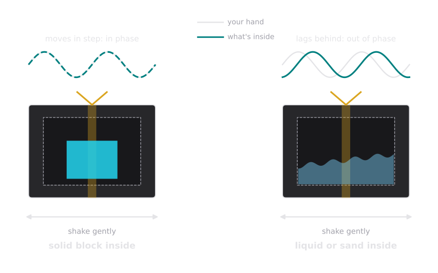
What to look for: the difference between the two boxes is not how far the content moves, but when. The time delay – the phase shift – is the key to everything in this article.

The Oscillation Test: Twisting Gently Back and Forth

In a rotational test (Part 2), the measuring plate keeps turning in one direction. In an oscillation test, it only turns back and forth by a tiny angle – typically well below one degree. The sample is deformed a little one way, a little the other way, over and over again, but never destroyed. That is the great advantage: you can study the inner structure of a material at rest, without shearing it apart.

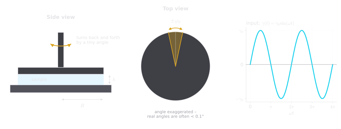
What to look for: the motion is tiny and smooth – a sine wave. The rheometer controls two things: how far it twists (the amplitude) and how fast it goes back and forth (the frequency).

The rheometer applies a sinusoidal strain and measures the stress:

$\gamma(t) = \gamma_0 \sin(\omega t), \qquad \tau(t) = \tau_0 \sin(\omega t + \delta)$

In words: the strain swings between $+\gamma_0$ and $-\gamma_0$ (the strain amplitude). How fast it swings is given by the angular frequency $\omega$ in rad/s. The stress swings with the same frequency, but with its own amplitude $\tau_0$ – and shifted in time by the phase angle $\delta$ (“delta”).

Frequency and angular frequency are related by $\omega = 2\pi f$: one full cycle per second ($f = 1$ Hz) corresponds to $\omega = 6.28$ rad/s.

Worked example. In a parallel-plate geometry, the strain at the rim is $\gamma = \varphi R/h$, where $\varphi$ is the twist angle in radians. With a plate radius $R = 12.5$ mm and a gap $h = 1$ mm, a strain amplitude of $\gamma_0 = 1\ \% = 0.01$ needs a twist of only $\varphi_0 = \gamma_0 h / R = 0.01 \times 1 / 12.5 = 0.0008$ rad – about 0.05°. You could not see this motion with your eyes.

The Phase Angle: Solid, Liquid or In Between?

Let us look at three ideal cases.

The ideal spring (Part 3) follows Hooke’s law, $\tau = G\gamma$. The stress is simply proportional to the strain: when the strain is largest, the stress is largest; when the strain is zero, the stress is zero. The two curves swing in step: $\delta = 0°$.

The ideal dashpot (Part 1) follows Newton’s law, $\tau = \eta\dot{\gamma}$. The stress is proportional to the speed of deformation. And the speed is largest when the plate passes through the middle position – exactly when the strain is zero. At the turning points, where the strain is largest, the plate stands still for a moment, and the stress is zero. The stress is shifted by a quarter of a cycle: $\delta = 90°$.

A viscoelastic material lies in between: $0° < \delta < 90°$.

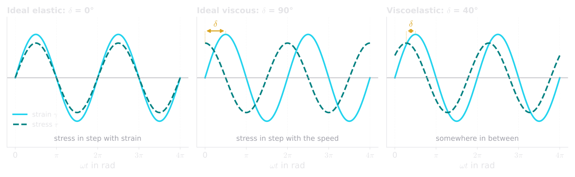
What to look for: compare where the peaks of the two curves are. The distance between them is the phase angle $\delta$ – the “delay” we felt when shaking the gift.

Phase angle $\delta$	Behavior	Example
0°	Ideal elastic – stress in step with strain	Steel spring, rubber
0° – 45°	Viscoelastic, solid-like ($G' > G''$)	Jelly, gel, crosslinked adhesive
45°	The border: elastic and viscous parts are equal	Gel point, crossover
45° – 90°	Viscoelastic, liquid-like ($G'' > G'$)	Polymer melt at low frequency
90°	Ideal viscous – stress in step with the speed	Water, honey

Everyday example – spring or spoon? Move a spoon back and forth through honey: you feel the strongest resistance in the middle of each stroke, where the spoon is fastest, and almost none at the turning points, where it briefly stops. Now pull a spring back and forth: the force is largest at the turning points, where it is stretched furthest, and zero in the middle. Same motion, different timing of the force – and the phase angle is nothing but this timing.

Storage Modulus and Loss Modulus

A phase angle between 0° and 90° means that the stress curve can be split into two parts: one that swings in step with the strain (the “spring” part) and one that swings in step with the speed (the “dashpot” part). Rheologists describe these two parts with two moduli:

$|G^*| = \frac{\tau_0}{\gamma_0}, \qquad G' = |G^*|\cos\delta, \qquad G'' = |G^*|\sin\delta$

$\tan\delta = \frac{G''}{G'}, \qquad |G^*| = \sqrt{G'^2 + G''^2}$

In words:

• $|G^*|$, the complex modulus, is the total stiffness – how much stress you get per unit of strain, regardless of timing.
• $G'$, the storage modulus (“G prime”), is the elastic part. It describes the energy the material stores during a cycle and gives back – like a spring.
• $G''$, the loss modulus (“G double prime”), is the viscous part. It describes the energy that is lost – turned into heat – in every cycle, like in a dashpot.
• $\tan\delta$, the loss factor, is the ratio of the two. Below 1, the material is solid-like; above 1, it is liquid-like.

All four quantities are measured in pascals, except $\tan\delta$, which has no unit.

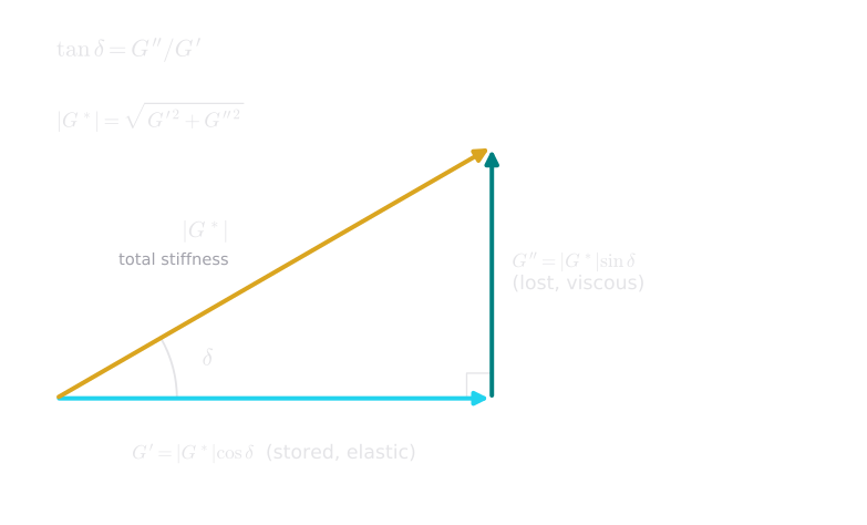
What to look for: $G'$ and $G''$ are simply the two sides of a right-angled triangle whose long side is the total stiffness. The phase angle sets how the total is divided between “stored” and “lost”.

For readers who like to see where this comes from: using the addition theorem for the sine,

$\tau(t) = \tau_0\sin(\omega t + \delta) = \gamma_0\left[\,G'\sin(\omega t) + G''\cos(\omega t)\,\right]$

In words: the measured stress is the sum of a part that follows the strain ($\sin\omega t$, weighted with $G'$) and a part that follows the speed of the strain ($\cos\omega t$, weighted with $G''$).

Worked example. A sample is deformed with $\gamma_0 = 1\ \%$. The rheometer measures a stress amplitude $\tau_0 = 50$ Pa and a phase angle $\delta = 30°$:

• $|G^*| = 50\ \mathrm{Pa} / 0.01 = 5000$ Pa
• $G' = 5000 \times \cos 30° \approx 4330$ Pa
• $G'' = 5000 \times \sin 30° = 2500$ Pa
• $\tan\delta = 2500/4330 \approx 0.58$ – below 1: the sample is solid-like.

Stored and Lost Energy

The names “storage” and “loss” are meant literally:

$W_{stored} = \tfrac{1}{2}\,G'\,\gamma_0^2, \qquad W_{lost} = \pi\,G''\,\gamma_0^2 \ \ \text{(per cycle)}$

In words: the energy stored at the maximum deformation – and returned on the way back – grows with $G'$. The energy converted into heat in every cycle grows with $G''$. Both are energies per volume of sample (J/m³).

For the worked example above: $W_{stored} = \tfrac{1}{2} \times 4330 \times 0.01^2 \approx 0.22$ J/m³ and $W_{lost} = \pi \times 2500 \times 0.01^2 \approx 0.79$ J/m³ per cycle.

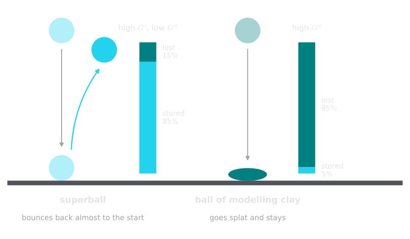
What to look for: the superball gives back almost all the energy of the fall – it is dominated by $G'$. The clay ball turns the energy into heat and deformation – it is dominated by $G''$.

There is an elegant way to see the lost energy directly: plot the stress against the strain over one cycle. The resulting loop is called a Lissajous figure, and the area enclosed by the loop is exactly the energy lost per cycle.

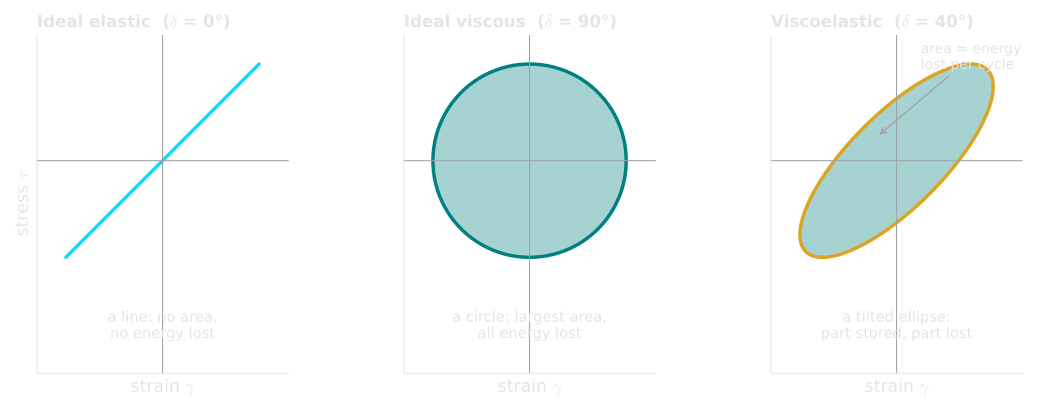
What to look for: the thinner the loop, the more elastic the material. A loop with no area at all is a perfect spring.

Try it at home – the wobble test: Put a jelly (or a panna cotta) on one plate and a spoonful of honey on another. Shake both plates gently from side to side. The jelly wobbles and springs back – it stores energy, $G' > G''$. The honey just smears along with the plate – it dissipates energy, $G'' > G'$. Now shake the jelly harder and harder until it cracks: you have just performed an amplitude sweep beyond the yield point.

Two Ways to Control the Test: CSD and CSS

Just as in rotational tests (Part 2), the rheometer can control either quantity:

• CSD – controlled shear deformation: the rheometer sets the strain amplitude $\gamma_0$ and measures the stress. This is the most common mode.
• CSS – controlled shear stress: the rheometer sets the stress amplitude $\tau_0$ and measures the strain. This is convenient for sensitive structures and for determining yield points in stress units.

Inside the linear range, both modes give identical values of $G'$ and $G''$ – they are two ways of asking the same question.

The Amplitude Sweep: How Hard Can You Shake?

The first oscillation test on any new sample is the amplitude sweep: the frequency is kept constant (often 10 rad/s), and the amplitude is increased step by step – from a whisper to a shout.

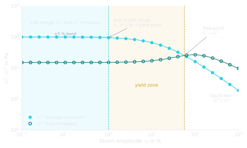
What to look for: three regions. On the left, the structure is untouched and both moduli are constant. In the middle, the structure starts to break. On the right, the material flows.

The amplitude sweep answers three questions:

• Where is the linear viscoelastic (LVE) range? As long as $G'$ and $G''$ do not change with amplitude, the test does not damage the sample. The end of this range, the limiting strain $\gamma_L$, is defined by a tolerance – typically where $G'$ has dropped by 5 %. Here: $\gamma_L \approx 1\ \%$. All further tests (like the frequency sweep) must stay below this strain.
• Where is the yield point? The stress at the end of the LVE range, $\tau_y = |G^*| \cdot \gamma_L$. Here: $\tau_y \approx 960\ \mathrm{Pa} \times 0.01 \approx 10$ Pa. Below this stress, the inner network of the gel is not damaged.
• Where is the flow point? The point where $G' = G''$ ($\delta = 45°$): from here on, the viscous part dominates and the material really flows. Here: at about 56 % strain, which corresponds to a stress of $\tau_f \approx 200$ Pa.

Between yield point and flow point lies the yield zone: the structure is already being damaged, but the material still behaves more like a solid than a liquid. Ketchup in a tilted bottle is in exactly this state just before it starts to move.

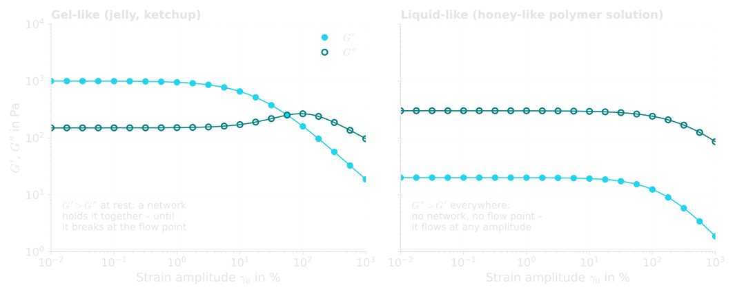
What to look for: only a material that is solid-like at rest ($G' > G''$) can have a flow point. A liquid-like material flows at every amplitude.

Common pitfall – skipping the amplitude sweep: Running a frequency sweep “at the usual 1 %” without checking the LVE range is one of the most frequent mistakes in the lab. If the chosen strain is outside the LVE range, the frequency sweep no longer describes the material at rest but a partly destroyed structure – and all conclusions drawn from it are questionable.

The Frequency Sweep: The Fingerprint of a Material

Once the LVE range is known, the second key test follows: the frequency sweep. The amplitude is fixed at a value well inside the LVE range, and the frequency is varied – typically from fast to slow, for example from 100 rad/s down to 0.01 rad/s.

Why vary the frequency? Because frequency is time in disguise. A frequency $\omega$ probes the material on a time scale of roughly

$t \approx \frac{1}{\omega}$

In words: a fast oscillation (high $\omega$) gives the material little time to rearrange – it shows its short-time behavior. A slow oscillation (low $\omega$) gives it plenty of time – it shows its long-time behavior. The frequency sweep is the Deborah number of Part 4 turned into a measurement.

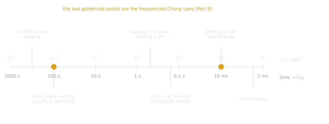
What to look for: slow frequencies stand for slow everyday processes, fast frequencies for fast ones. The two goldenrod points – 0.01 and 100 rad/s – are the “bonding” and the “debonding” time scales of an adhesive tape.

What a Single Maxwell Element Does

The simplest viscoelastic liquid, the Maxwell model with modulus $G$ and relaxation time $\lambda$ (Parts 4 and 6), gives

$G'(\omega) = G\,\frac{(\omega\lambda)^2}{1+(\omega\lambda)^2}, \qquad G''(\omega) = G\,\frac{\omega\lambda}{1+(\omega\lambda)^2}$

In words: at low frequencies ($\omega\lambda \ll 1$), the material has time to relax – it flows, and $G'' > G'$. At high frequencies ($\omega\lambda \gg 1$), it has no time to relax – it behaves like a spring, and $G' > G''$, with $G'$ approaching $G$. The two curves cross exactly where $\omega = 1/\lambda$: at the crossover, both moduli equal $G/2$.

Worked example. Silly Putty with $G = 10^5$ Pa and $\lambda = 1$ s has its crossover at $\omega_c = 1$ rad/s, which is about 0.16 Hz – a slow back-and-forth every six seconds. Knead it faster and it feels rubbery; slower, and it feels like dough.

Reading a Real Frequency Sweep

A real polymer melt contains many relaxation times – the “orchestra” of Part 6 – and its frequency sweep shows several characteristic zones:

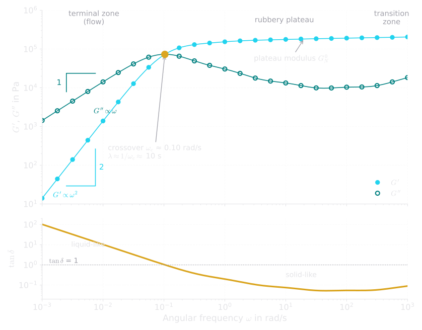
What to look for: read the plot from right to left, from fast to slow. At fast frequencies the melt is rubbery; at slow frequencies it flows. The crossover marks the border – and gives the longest relaxation time.

• Terminal zone (low $\omega$): the material flows. $G'' > G'$, and the curves follow characteristic slopes: $G' \propto \omega^2$ and $G'' \propto \omega$ (slopes 2 and 1 on log–log axes). Here, the zero-shear viscosity can be read directly: $\eta_0 = \lim_{\omega \to 0} G''/\omega$. For our melt: $G''(0.001\ \mathrm{rad/s}) \approx 1430$ Pa, so $\eta_0 \approx 1.4 \times 10^6$ Pa·s.
• Crossover: $G' = G''$ at $\omega_c \approx 0.1$ rad/s. Its inverse, $1/\omega_c \approx 10$ s, is a good estimate of the longest relaxation time of the material.
• Rubbery plateau: $G'$ is almost constant, and $G' \gg G''$. The entanglements between the long chains act like temporary crosslinks – a network that holds only as long as the chains have no time to slide out of it. The height of the plateau, the plateau modulus $G_N^0$, tells how dense this network is: $G_N^0 \approx \rho R T / M_e$, where $M_e$ is the molar mass between two entanglements. With $G_N^0 \approx 2\times10^5$ Pa, a density of 1000 kg/m³ and $T = 298$ K, this gives $M_e \approx 12$ kg/mol.
• Transition zone (high $\omega$): at still higher frequencies, even short chain segments cannot follow; $G''$ rises again, and eventually the material becomes glassy. Because rheometers cannot oscillate arbitrarily fast, this region is usually reached by cooling the sample instead – the idea of time–temperature superposition in Part 8.

Every Material Has Its Own Fingerprint

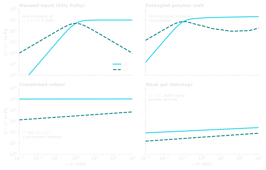
What to look for: a liquid always ends with $G'' > G'$ at low frequencies; a solid or gel keeps $G' > G''$ down to the slowest frequency.

Material	Low frequencies	Crossover	High frequencies
Maxwell liquid	$G'' > G'$, slopes 1 and 2	one, at $1/\lambda$	$G'$ constant, $G''$ falls
Entangled melt	$G'' > G'$ (flows)	at $\approx 1/\lambda_{max}$	rubbery plateau
Crosslinked rubber	$G' \gg G''$, flat	none	$G' \gg G''$, flat
Weak gel	$G' > G''$, nearly parallel	none	both rise slowly

In the lab – the gel point: When a liquid turns into a solid – a resin curing, a gelatin solution cooling – there is a special moment in between: the gel point. At this moment, $G'$ and $G''$ run parallel over the whole frequency range, and $\tan\delta$ does not depend on frequency (Winter–Chambon criterion). In a series of frequency sweeps during curing, the gel point is where the $\tan\delta$ curves of all frequencies cross in one point.

A Recipe for Good Oscillation Measurements

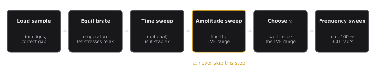
What to look for: the amplitude sweep comes before the frequency sweep – always.

In the lab – good oscillation practice:

• Loading: trim excess sample at the edge; underfilled or overfilled gaps give wrong moduli. For adhesives, parallel plates of 8 mm or 25 mm diameter are typical.
• Equilibrate: give the sample time to reach the test temperature and to relax the stresses from loading (Part 6).
• Time sweep: at constant amplitude and frequency, check whether $G'$ and $G''$ stay constant. Drying, curing or settling show up as a drift.
• Amplitude sweep: find $\gamma_L$; for the frequency sweep, choose an amplitude well inside the LVE range (often a factor of 2–5 below $\gamma_L$).
• Frequency sweep: from high to low frequency; low frequencies take long – one cycle at 0.01 rad/s lasts more than ten minutes.

Why It Matters for Adhesives

A pressure-sensitive adhesive must behave like a liquid when it is pressed on – to flow into the roughness of a surface within seconds – and like a solid when it is peeled off within milliseconds. The frequency sweep shows both faces at once: the low frequencies stand for bonding, the high frequencies for debonding.

In Part 8 we will build the Chang Viscoelastic Window from just four numbers read from a frequency sweep: $G'$ and $G''$ at 0.01 rad/s and at 100 rad/s. The three model tapes of Parts 5 and 6 already give a first taste at the slow end:

Model tape	$G'$ at 0.01 rad/s	$G''$ at 0.01 rad/s	Character at slow time scales
Tape A – removable label	≈ 3,300 Pa	≈ 3,900 Pa	$G'' > G'$: liquid-like, creeps off under load
Tape B – general purpose	≈ 17,000 Pa	≈ 11,000 Pa	solid-like, balanced
Tape C – high-shear mounting	≈ 63,000 Pa	≈ 10,000 Pa	clearly solid-like, holds loads for a long time

(Model data, based on the model tapes of Parts 5 and 6 – the same values are used in Part 8.) The ranking is the same as for the holding times in Part 5 – three different tests, one consistent picture.

Key Takeaways

• Oscillation tests probe a material gently, without destroying its structure – like shaking a wrapped gift.
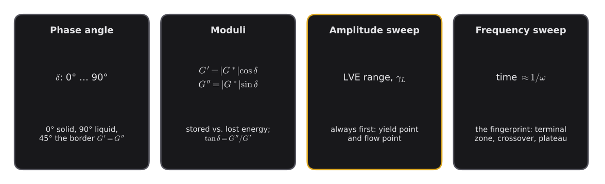
• The phase angle $\delta$ tells the character at a glance: 0° solid, 90° liquid, 45° the border where $G' = G''$.
• $G'$ (storage modulus) measures the stored, elastic part; $G''$ (loss modulus) the lost, viscous part; $\tan\delta = G''/G'$.
• Always run an amplitude sweep first: it gives the LVE range, the yield point and the flow point.
• A frequency sweep is the fingerprint of a material: terminal zone, crossover ($\approx 1/\lambda$) and rubbery plateau reveal its time scales and its network.
• Frequency is time in disguise: 0.01 rad/s ≈ 100 s (bonding), 100 rad/s ≈ 10 ms (peeling) – the two frequencies of the Chang window.

Key Terms

Term	Meaning in plain language	Symbol, unit
Oscillation test	Twisting the sample gently back and forth	–
Strain amplitude	Largest deformation in each cycle	$\gamma_0$, – or %
Angular frequency	How fast the sample is twisted back and forth	$\omega$, rad/s
Phase angle	Time delay between stress and strain	$\delta$, °
Complex modulus	Total stiffness	$\lvert G^* \rvert$, Pa
Storage modulus	Elastic, stored part	$G'$, Pa
Loss modulus	Viscous, lost part	$G''$, Pa
Loss factor	Ratio of lost to stored	$\tan\delta$, –
Lissajous figure	Stress plotted against strain over one cycle	–
LVE range	Range of amplitudes that does not damage the structure	up to $\gamma_L$
Yield point	Stress at the end of the LVE range	$\tau_y$, Pa
Flow point	Point where $G' = G''$ in an amplitude sweep	$\tau_f$, Pa
Crossover	Frequency where $G' = G''$ in a frequency sweep	$\omega_c$, rad/s
Terminal zone	Low frequencies where the material flows	–
Rubbery plateau	Range where $G'$ is almost constant	$G_N^0$, Pa
Gel point	Transition from liquid to solid; $\tan\delta$ independent of $\omega$	–

Coming Up Next

A sticky note comes off cleanly and can be used again. Packaging tape holds a heavy box for months. A freezer label has to grab instantly, even at −20 °C. All three are pressure-sensitive adhesives – yet each needs a different balance between flowing and resisting. In Part 8 we use the frequency sweep to draw the Chang Viscoelastic Window: a simple map that shows at a glance what an adhesive is good for – and how a formulator can move it.

References

1. Mezger, T. G.: The Rheology Handbook, 5th ed., Vincentz Network, Hanover 2020.
2. Macosko, C. W.: Rheology: Principles, Measurements, and Applications, Wiley-VCH, New York 1994.
3. Ferry, J. D.: Viscoelastic Properties of Polymers, 3rd ed., Wiley, New York 1980.
4. Barnes, H. A.; Hutton, J. F.; Walters, K.: An Introduction to Rheology, Elsevier, Amsterdam 1989.
5. Winter, H. H.; Chambon, F.: Analysis of linear viscoelasticity of a crosslinking polymer at the gel point, Journal of Rheology 30 (1986) 367–382.
6. Chang, E. P.: Viscoelastic windows of pressure-sensitive adhesives, The Journal of Adhesion 34 (1991) 189–200.