6 Stress Relaxation: How Materials Forget a Deformation
Why does a rubber band around old letters lose its grip while staying just as stretched? An illustrated introduction to the relaxation test, the relaxation modulus, relaxation times and the relaxation spectrum – and what they reveal about adhesive tapes.
Wrap a rubber band tightly around a bundle of letters and it grips them firmly. Put the bundle in a drawer and find it again ten years later: the band is still stretched to exactly the same length – it has not moved at all – but now it hardly holds anything. You can pull the letters out with two fingers. The deformation stayed the same, but the force faded away.
This fading of force at constant deformation is called stress relaxation. It is the mirror image of creep, which we met in Part 5: there the load was constant and the deformation grew; here the deformation is constant and the load shrinks. You know it from a hair tie that gets loose over the day, from a screw in a plastic housing that has to be retightened, or from cling film that no longer pulls tight over a bowl after a few hours in the fridge.
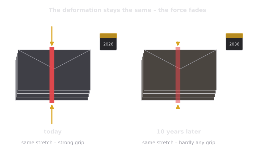
What to look for: the band has the same length in both pictures. Only the arrows – the force with which it squeezes the letters – have shrunk.
Everyday example – honest small print: In a real rubber band, oxygen and light also slowly break the rubber molecules, which helps the band to lose its grip. But even a perfectly protected band relaxes: its chains slowly rearrange into a less stressed state. That physical part is what this article is about.
The Relaxation Test: Constant Deformation, Fading Stress
The test is as simple as the creep test, just the other way round:
- At time , the rheometer deforms the sample to a strain – as fast as it possibly can.
- It then holds this deformation constant, like the rubber band that stays stretched around the letters.
- It records the stress that is needed to keep the sample in its deformed shape.
Because the rheometer now controls the deformation, this is a test in controlled shear deformation (CSD) mode.
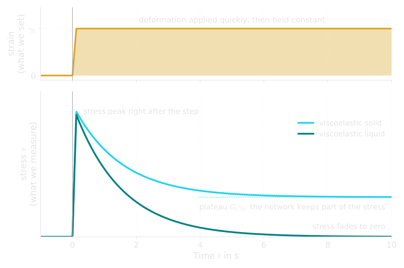
What to look for: the input (top) never changes after the step. Yet the output (bottom) keeps falling – the material “gets used to” its new shape and needs less and less force to stay there.
The Relaxation Modulus: Stiffness Over Time
As in the creep test, we want a number that does not depend on how far we deformed the sample. So we divide the stress by the strain and get the relaxation modulus:
In words: the relaxation modulus is the stress needed per unit of deformation after time . It is the shear modulus of Part 3 – but now it has a clock attached. Its unit is the pascal (Pa). A large means the material still resists strongly; a small one means it has largely “forgotten” that it was deformed.
Worked example. A sample is sheared to . Right after the step, the rheometer needs a stress of 1000 Pa; after 20 s, only 230 Pa. So kPa and kPa. Within 20 seconds, the material has lost more than three quarters of its stiffness.
As with creep, the division only makes sense in the linear viscoelastic range: must come out the same whether you deform the sample by 0.5 % or by 1 %. At large deformations, the curves drop faster and lower – the deformation itself damages the inner structure, and is no longer a pure material property.
Four Ways to Relax
Let us start again with the ideal materials. Their relaxation curves are just as different as their creep curves.
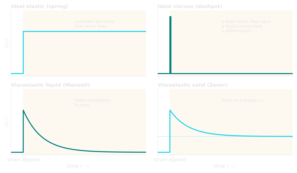
What to look for: the long-time end tells you what kind of material you have. Does the curve go to zero (a liquid) or to a plateau (a solid)?
| Material | Relaxation modulus | Everyday example |
|---|---|---|
| Ideal elastic (spring) | Constant – it never tires | Steel spring |
| Ideal viscous (dashpot) | A short spike during the step, then zero | Water, honey |
| Viscoelastic liquid | Fades completely to zero | Silly Putty, polymer melts, most tape adhesives |
| Viscoelastic solid | Fades to a plateau, the equilibrium modulus | Crosslinked rubber, gels, memory foam |
Why does the ideal liquid show only a spike? A liquid needs force only while it is being moved. As soon as the deformation stops, honey happily stays in its new shape without any force at all – it has no memory of where it came from. A crosslinked rubber, on the other hand, is held together by a permanent network (Part 3). Its chains can rearrange locally, but the network as a whole keeps pulling back: part of the stress remains forever.
Quick check: You deform a jelly and hold it. After an hour, the stress has dropped to 40 % of its initial value and no longer changes. Liquid or solid? (Solid – it keeps a plateau. Its equilibrium modulus is 40 % of the initial modulus.)
One Relaxation Time: The Maxwell Decay
The simplest viscoelastic liquid is the Maxwell model from Part 4: a spring and a dashpot connected in series. Right after the step, only the spring is stretched – the dashpot has had no time to move – and the full stress appears. Then the dashpot slowly gives way, the spring shortens, and the stress fades:
In words: the stress fades by the same fraction in every time interval , the relaxation time. After one , 36.8 % of the initial stress is left; after another , 36.8 % of that; and so on. It is the same rule that governs radioactive decay or a cup of coffee cooling down.
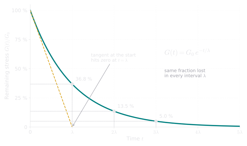
What to look for: two quick ways to find – read the time at which 37 % is left, or draw the tangent at the start and see where it hits zero.
| Time | Remaining stress |
|---|---|
| 36.8 % | |
| 13.5 % | |
| 5.0 % | |
| 0.7 % |
If you prefer “half-lives”: half of the stress is gone after .
Worked example. A melt relaxes from kPa to kPa. For a single relaxation time, the ratio of two values depends only on the time between them:
The Semilog Test: Is It Really Just One Time?
A neat trick reveals whether a material has one relaxation time or many: plot on a logarithmic vertical axis against a linear time axis. An exponential decay then becomes a straight line whose steepness is set by (in natural-logarithm units, the slope is exactly ).
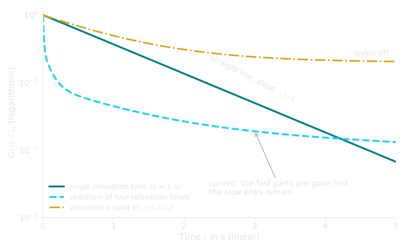
What to look for: only one of the three curves is straight. The curved one is the normal case for real polymers – it is the fingerprint of many relaxation times.
Real polymers almost never give a straight line. Their curve first drops steeply and then flattens out: the fast parts of the material have already relaxed, while slow parts are still holding on. To describe this, we need more than one relaxation time.
Many Relaxation Times: The Relaxation Orchestra
A polymer chain is not a single spring. It is a long, entangled molecule with structures of all sizes: a few neighboring chain segments can rearrange within microseconds, a longer section in milliseconds, and a whole chain, snaking its way out of the tangle of its neighbors, may need seconds, hours or longer.
Each group of structures behaves like its own little Maxwell element with its own modulus and its own relaxation time . Put them all in parallel and you get the generalized Maxwell model:
In words: the total relaxation modulus is the sum of many individual decays – plus, for a solid, the permanent plateau (for a liquid, ). The set of pairs is called the relaxation spectrum.
Think of it as an orchestra. At the start, all instruments play together – that is the full initial stiffness. The piccolos (short chain segments) stop first, then the violins, then the cellos, and at the very end only the double basses (whole chains) are still humming. What you hear at any moment is the sum of the instruments still playing.
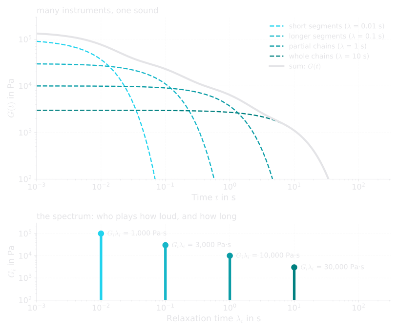
What to look for: every single mode falls off a cliff within about one decade of time. Only together do they produce the long, gentle slope of a real polymer.
On log–log axes, the difference between one relaxation time and a whole spectrum becomes even more striking:
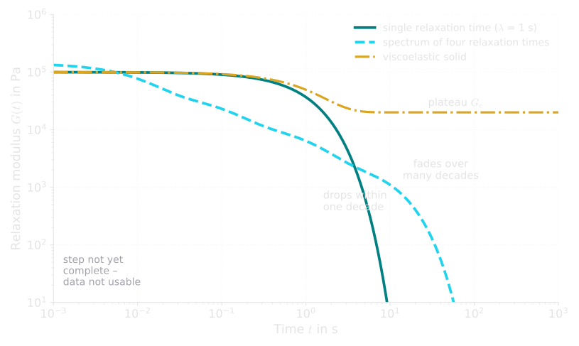
What to look for: a single Maxwell element “dies” within one decade of time. A real polymer relaxes over many decades – which is why rheologists love logarithmic time axes.
Notice the shaded region on the left: it hides the fastest mode of our spectrum (0.01 s). A real rheometer cannot switch on a deformation infinitely fast. That is a first hint why fast relaxation processes are usually measured with oscillation instead – more on that in Part 7.
The Zero-Shear Viscosity: The Area Under the Curve
Relaxation and flow are closely related. Every time a Maxwell element relaxes, its dashpot has flowed. It turns out that the zero-shear viscosity – the viscosity at rest, which we determined from the final slope of the creep curve in Part 5 – is simply the area under the relaxation curve:
In words: add up how much stiffness the material has, multiplied by how long it keeps it. A stiff material that relaxes quickly and a soft material that relaxes slowly can have the same . For a single mode, the area under the exponential is exactly the rectangle .
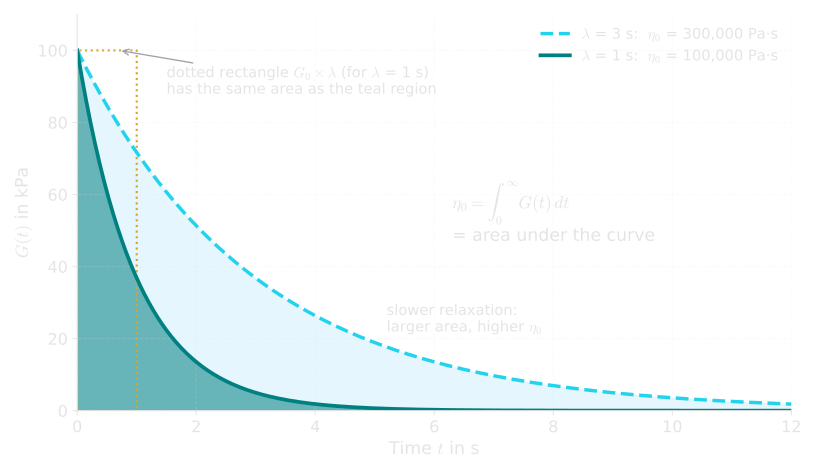
What to look for: same starting stiffness, three times the relaxation time, three times the area – and three times the zero-shear viscosity.
Worked example. For the four-mode spectrum of the orchestra figure:
The slowest mode, the one with the smallest modulus, contributes more than two thirds of the viscosity. The double basses are quiet, but they play the longest – and that is what counts for flow.
Common pitfall – ignoring the tail: Because the slowest modes dominate , stopping a relaxation test too early cuts off exactly the part of the area that matters most. At long times, the stress becomes tiny and drowns in instrument noise. If the tail cannot be measured, creep (Part 5) is usually the better way to get .
Creep and Relaxation: Two Sides of One Coin
Creep and relaxation are not two different material properties. They are two views of the same inner behavior – just asked differently:
- Creep asks: How far does it go under a fixed load?
- Relaxation asks: How much force is still needed to hold a fixed deformation?
Let us test this with Tape B, the general-purpose tape adhesive we characterized in Part 5 with the Burgers model (, , s, Pa·s). The same four-element model can be translated into a relaxation modulus. It turns out to be a small orchestra of just two instruments:
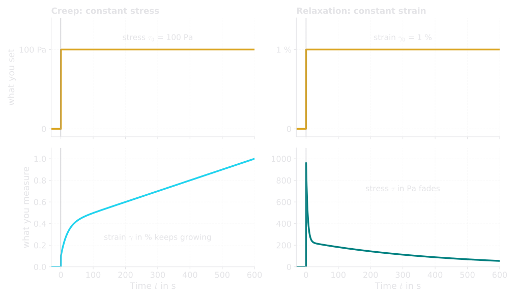
What to look for: the fast drop of the relaxation curve and the bend in the creep curve are the same inner process (the 4.8 s mode); the slow tail of the relaxation curve and the straight creep slope are the same flow (the 415 s mode).
Two checks show that these really are the same material:
- Instant stiffness: kPa – exactly , the inverse of the instant creep compliance.
- Zero-shear viscosity: Pa·s – exactly the Pa·s we read from the creep slope. The slow mode supplies 96 % of it.
And the mean relaxation time s that we calculated at the end of Part 5? It sits right next to the slowest mode of 415 s. Everything fits together.
Three Tapes, Three Memories
Now we can translate all three model adhesives of this series from their creep curves (Part 5) into relaxation curves:
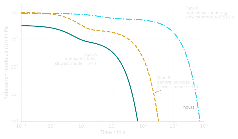
What to look for: the three tapes differ less in their starting stiffness than in how long they keep it. Tape C still “remembers” its deformation after hours.
- Tape A forgets quickly. Stresses in the adhesive are gone within minutes – ideal for a label that should conform to a surface and come off cleanly, but also the reason it cannot carry a permanent load.
- Tape B keeps part of its stiffness for several minutes – a balanced memory.
- Tape C holds on to its stiffness for hours. Its slowest mode (about 2.4 hours) acts almost like a permanent plateau. A strongly crosslinked mounting tape would keep a true plateau forever – it would be a viscoelastic solid.
In the lab – good relaxation practice:
- Rise time: no motor can apply a deformation instantly. A real step takes roughly 10 to 100 milliseconds. During this time and for several rise times afterwards, the data are not reliable – so the fastest relaxation processes are out of reach.
- Linear range: choose small enough that does not depend on it. Check with a second, smaller strain.
- Signal at long times: as the stress fades, it approaches the resolution limit of the torque sensor. A large measuring geometry helps.
- Temperature: relaxation times of polymers change strongly with temperature – often by a factor of two or more for a change of just a few kelvin. Keep the temperature constant and let the sample equilibrate before the step.
- From oscillation: in practice, the spectrum is usually not taken from a step test but calculated by the rheometer software from a frequency sweep (Part 7), typically with about one mode per decade of time.
Try it at home – the tired rubber band: Take two identical rubber bands from the same pack. Wrap one tightly around a thick book; keep the other loose in a drawer. After a week, remove the first band and lay both side by side. The stretched one is longer at rest and feels looser: part of its tension has relaxed – and part of the deformation has become permanent.
A Look Ahead: From Relaxation to Oscillation
The relaxation spectrum is the “genetic code” of a viscoelastic material. Once you know it, you can predict how the material responds to any kind of deformation – creep, relaxation, or the periodic back-and-forth of an oscillation test. As a preview of Part 7, here is how the same spectrum predicts the two oscillation moduli at an angular frequency :
In words: modes whose relaxation time is long compared with the oscillation period () have no time to relax and act like springs – they contribute to the storage modulus . Modes whose relaxation time matches the period () dissipate the most energy – they dominate the loss modulus . Don’t worry if these formulas look heavy: Part 7 unpacks them step by step.
Why It Matters for Adhesives
For a pressure-sensitive adhesive, the relaxation spectrum is like a timetable of its behavior:
- The slow modes (seconds to hours) decide how the adhesive behaves under a permanent load: cohesion, holding power, and the resistance to creeping off a wall. They correspond to the low-frequency corner of the Chang Viscoelastic Window in Part 8.
- The fast modes (milliseconds) decide what happens when the tape is peeled off quickly: how much energy is dissipated and how strong the peel force is. They correspond to the high-frequency corner of the window.
- Relaxation after bonding: when a tape is pressed onto a rough surface, the adhesive is squeezed into the valleys and stores stress. As this stress relaxes, the adhesive keeps flowing into closer contact. That is one reason why the peel force of many tapes increases with dwell time – and why peel test standards specify how long to wait after application, typically 20 minutes and 24 hours.
- Tapes applied under tension, for example pulled tight around a cable bundle or a box, keep a stress in the backing. If the adhesive cannot relax it, the tape ends slowly lift.
In Part 9, individual features of the spectrum – such as the modulus at 0.01 rad/s or the area under at high frequencies – become inputs for a machine-learning model that predicts peel adhesion.
Key Takeaways
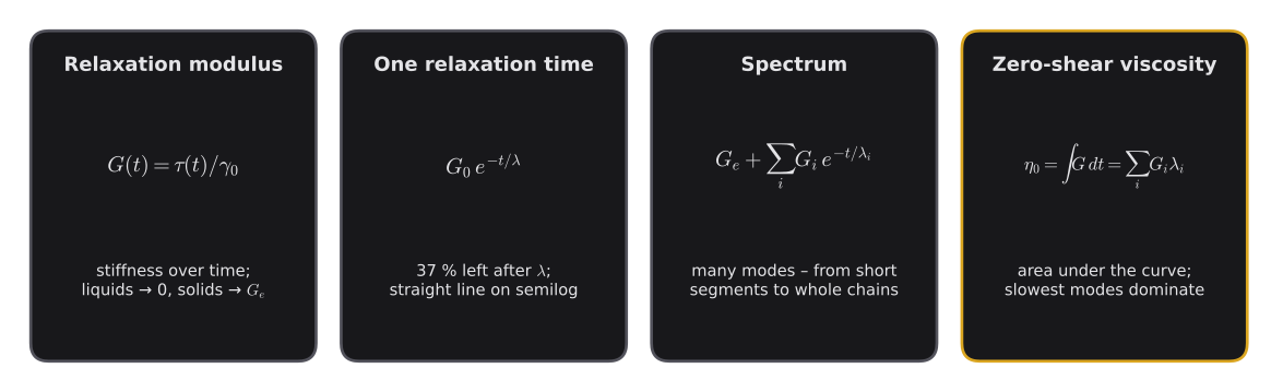
- In a relaxation test, a deformation is applied quickly and held constant, and the fading stress is recorded: .
- Liquids relax completely (); solids keep an equilibrium modulus .
- A single relaxation time gives an exponential decay: after one , 37 % of the stress is left; on a semilog plot it is a straight line.
- Real polymers need a spectrum of relaxation times – an orchestra of Maxwell elements that fall silent one after another.
- The zero-shear viscosity is the area under the relaxation curve, – dominated by the slowest modes.
- Creep, relaxation and oscillation describe the same material – the spectrum connects them.
Key Terms
| Term | Meaning in plain language | Symbol, unit |
|---|---|---|
| Stress relaxation | Fading of stress at constant deformation | – |
| Relaxation modulus | Stress per unit of strain after time – “stiffness over time” | , Pa |
| Relaxation time | Time after which 37 % of the stress is left | , s |
| Equilibrium modulus | Stiffness a solid keeps forever | , Pa |
| Maxwell model | Spring and dashpot in series – one relaxation time | – |
| Zener model | Maxwell element plus a parallel spring – a viscoelastic solid | – |
| Generalized Maxwell model | Many Maxwell elements in parallel | – |
| Relaxation spectrum | The set of moduli and relaxation times | |
| Mode | One Maxwell element of the spectrum | , |
| Zero-shear viscosity | Area under the relaxation curve | , Pa·s |
| Rise time | Time the rheometer needs to apply the step | s |
| Semilog plot | Logarithmic vertical axis, linear time axis | – |
Coming Up Next
Before opening a wrapped present, you shake it gently: a solid block moves exactly with your hand, while sand or liquid lags behind and sloshes. Shaking tells you a lot about what is inside – without opening or breaking anything. In Part 7 we do exactly this with a rheometer: the oscillation test twists the sample gently back and forth and listens to how the resisting force follows. We will see how this splits a material’s behavior neatly into an elastic part and a viscous part – and why it has become the most important test in rheology.
References
- Mezger, T. G.: The Rheology Handbook, 5th ed., Vincentz Network, Hanover 2020.
- Macosko, C. W.: Rheology: Principles, Measurements, and Applications, Wiley-VCH, New York 1994.
- Ferry, J. D.: Viscoelastic Properties of Polymers, 3rd ed., Wiley, New York 1980.
- Tschoegl, N. W.: The Phenomenological Theory of Linear Viscoelastic Behavior, Springer, Berlin 1989.
- Dealy, J. M.; Read, D. J.; Larson, R. G.: Structure and Rheology of Molten Polymers, 2nd ed., Hanser, Munich 2018.
- FINAT: FINAT Test Method No. 1 – Peel Adhesion (180°) at 300 mm per Minute, FINAT Technical Handbook, The Hague.