4 Viscoelasticity and Normal Stress Differences

Throw a ball of Silly Putty on the floor and it bounces back like a rubber ball. Leave the same ball on the table overnight and the next morning you find a flat puddle. Memory foam does something different: press your hand into it and it gives way slowly; take your hand away and the imprint disappears – slowly, but completely.

Neither material is a simple liquid, and neither is a simple solid. They are viscoelastic: part spring, part dashpot. In Part 1 we met the dashpot, the symbol of flow; in Part 3 the spring, the symbol of elasticity. This article combines the two – and shows a spectacular consequence of elasticity in flowing liquids: dough that climbs up a rotating rod.

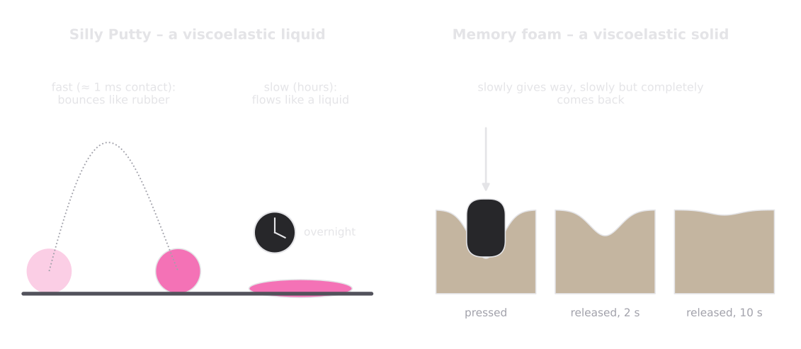
What to look for: Silly Putty behaves like a solid on short time scales and like a liquid on long ones. Memory foam always returns to its shape – it just takes its time.

Solid or Liquid? It Depends on How Long You Watch

The key to viscoelasticity is time. Every viscoelastic material has an internal time scale – its relaxation time $\lambda$ (“lambda”). You can think of it as the material’s memory time: how long it takes to “forget” a deformation and rearrange its inner structure.

Whether a material appears solid or liquid depends on how its memory time compares with the time we watch it. This ratio is called the Deborah number:

$De = \frac{\lambda}{t_{obs}}$

In words: $De$ is the material’s relaxation time divided by the observation time $t_{obs}$. If $De$ is much larger than 1, the material has no time to rearrange during the observation – it behaves like a solid. If $De$ is much smaller than 1, it has plenty of time – it behaves like a liquid.

Worked example. Silly Putty has a relaxation time of roughly one second. During a bounce, the ball touches the floor for about a millisecond: $De \approx 1\ \mathrm{s} / 0.001\ \mathrm{s} = 1000$ – solid, it bounces. Overnight ($t_{obs} \approx 30{,}000$ s): $De \approx 0.00003$ – liquid, it flows.

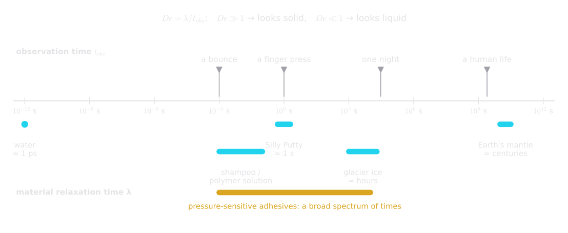
What to look for: compare a material with an observation time. Where the material’s time lies far to the right of the observation, it appears solid; far to the left, it appears liquid.

The ruler contains a surprising example: the rock of the Earth’s mantle. For earthquake waves, which last seconds, it behaves like an elastic solid. Over tens of thousands of years, it flows – the land in Scandinavia is still rising today because the mantle underneath slowly flows back after the heavy ice sheets of the last ice age melted.

Everyday example – where the name comes from: The Deborah number was named in 1964 by the rheologist Markus Reiner after the prophetess Deborah in the Bible, who sang: “The mountains flowed before the Lord.” Reiner’s point: given enough time – God’s time scale – even mountains flow. Everything flows; the question is only how long you watch.

Try it at home – Silly Putty: Roll a ball of Silly Putty (or bouncing putty) and drop it: it bounces. Now pull it apart slowly with both hands: it stretches into long threads like honey. Pull it apart with a sudden jerk: it snaps with a clean break, like a solid. Same material, three different behaviors – only the speed has changed.

Two Building Blocks, Two Ways to Combine Them

To describe viscoelastic materials, we combine the spring (elasticity, drawn in cyan) and the dashpot (flow, drawn in teal). There are two simple ways to do this: one behind the other (in series) or side by side (in parallel).

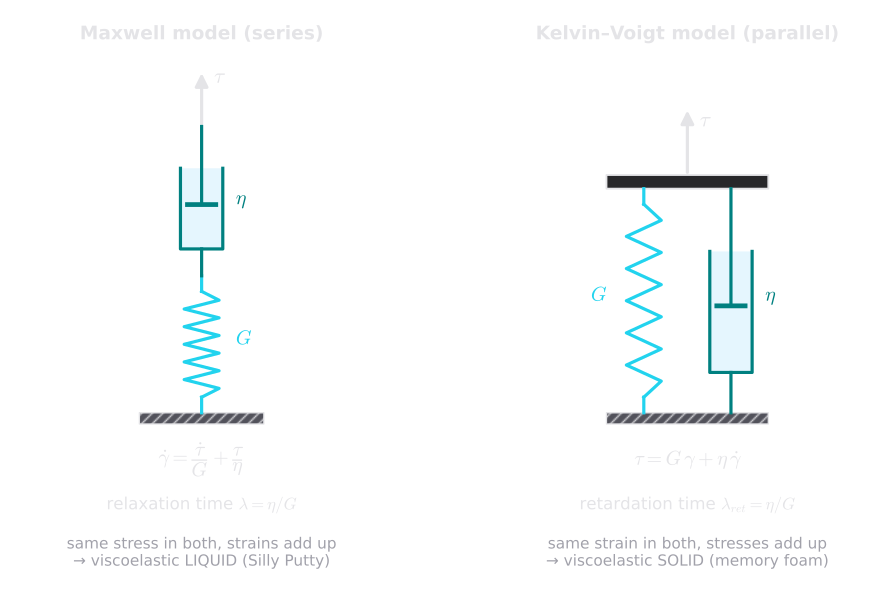
What to look for: in series, both elements carry the same force, and their deformations add up. In parallel, both elements are deformed by the same amount, and their forces add up.

The Maxwell Model: Spring and Dashpot in Series

In the Maxwell model, the spring and the dashpot are connected one behind the other. Its equation can be derived in three steps:

1. The total deformation is the sum of the spring’s and the dashpot’s deformation: $\gamma = \gamma_{spring} + \gamma_{dashpot}$.
2. Taking the rate of change on both sides: $\dot{\gamma} = \dot{\gamma}_{spring} + \dot{\gamma}_{dashpot}$.
3. The spring follows Hooke’s law, $\gamma_{spring} = \tau/G$, so its rate is $\dot{\tau}/G$. The dashpot follows Newton’s law, so its rate is $\tau/\eta$. Both carry the same stress $\tau$. Together:

$\dot{\gamma} = \frac{\dot{\tau}}{G} + \frac{\tau}{\eta}$

In words: the total deformation rate is the stretching rate of the spring plus the flow rate of the dashpot. The ratio of the two material constants defines the relaxation time:

$\lambda = \frac{\eta}{G}$

What happens after a sudden stretch? Imagine stretching a Maxwell element suddenly and then holding its total length fixed. In the first instant, only the spring can react – the dashpot needs time to move. The spring is stretched and pulls with full force. Then the dashpot slowly gives way, the spring shortens, and the force fades.

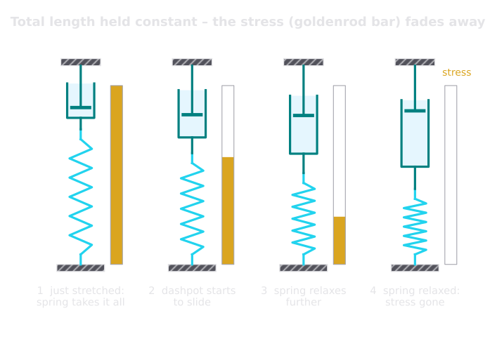
What to look for: the total length never changes, yet the stress (goldenrod bar) disappears – the deformation is gradually “handed over” from the spring to the dashpot.

Mathematically: with the total length held constant, $\dot{\gamma} = 0$, and the Maxwell equation becomes $\dot{\tau} = -\tau/\lambda$. The stress decreases at a rate proportional to its current value. Separating the variables ($d\tau/\tau = -dt/\lambda$) and integrating gives

$\tau(t) = G\,\gamma_0\,e^{-t/\lambda}$

In words: the stress fades exponentially. After one relaxation time $\lambda$, only 37 % of the initial stress is left; after three relaxation times, only 5 %. This process is called stress relaxation, and it is the subject of Part 6.

What happens under a constant load? If we pull on a Maxwell element with a constant stress $\tau_0$, the spring stretches instantly by $\tau_0/G$, and then the dashpot flows at a constant rate $\tau_0/\eta$:

$\gamma(t) = \frac{\tau_0}{G} + \frac{\tau_0}{\eta}\,t$

In words: an instant elastic jump, then endless flow. When the load is removed, the spring snaps back, but the flow of the dashpot remains as a permanent deformation. A Maxwell material is therefore a viscoelastic liquid – just like Silly Putty.

Worked example. A Silly-Putty-like material with $G = 10^5$ Pa and $\eta = 10^5$ Pa·s has a relaxation time of $\lambda = 10^5 / 10^5 = 1$ s. Stretched suddenly and held, its stress drops to 37 % after 1 s and to 5 % after 3 s.

The Kelvin–Voigt Model: Spring and Dashpot in Parallel

In the Kelvin–Voigt model, spring and dashpot sit side by side between two rigid bars. Both are deformed by exactly the same amount, and the load is shared between them:

$\tau = G\,\gamma + \eta\,\dot{\gamma}$

In words: the total stress is the spring’s share (proportional to the deformation) plus the dashpot’s share (proportional to the deformation rate). The characteristic time is called the retardation time, $\lambda_{ret} = \eta/G$, because it describes how much the dashpot delays the spring.

What happens under a constant load? When a constant stress $\tau_0$ is applied, the spring would like to jump to its final length $\tau_0/G$ immediately, but the dashpot holds it back. Rearranging the equation gives $\dot{\gamma} = (\tau_0 - G\gamma)/\eta$: the deformation speed is proportional to the distance still remaining to the final value. That is again the recipe for an exponential curve:

$\gamma(t) = \frac{\tau_0}{G}\left(1 - e^{-t/\lambda_{ret}}\right)$

In words: the material gives way quickly at first, then more and more slowly, and approaches the final deformation $\tau_0/G$ without ever flowing beyond it. When the load is removed, the spring pulls everything back – slowly, because the dashpot brakes it, but completely. A Kelvin–Voigt material is a viscoelastic solid – like memory foam.

Worked example. A memory foam with $G = 5$ kPa and $\eta = 5 \times 10^4$ Pa·s has a retardation time of $\lambda_{ret} = 10$ s. After 10 s under a constant load, it has reached 63 % of its final deformation; after 30 s, 95 %. After release, it needs about the same time to recover.

The difference between the two models becomes clear when we load both in the same way:

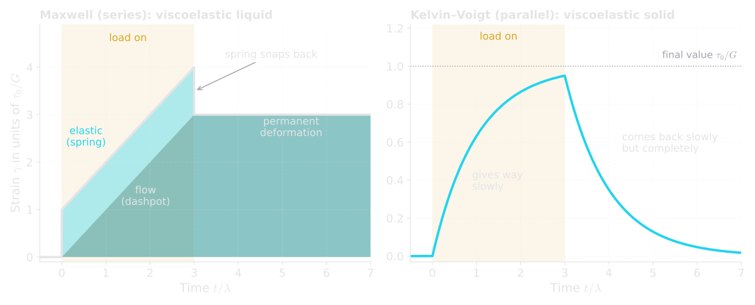
What to look for: the Maxwell liquid keeps a permanent deformation (teal); the Kelvin–Voigt solid returns to zero. Both responses take time – that is what makes them viscoelastic.

And when we stretch both suddenly and hold the deformation:

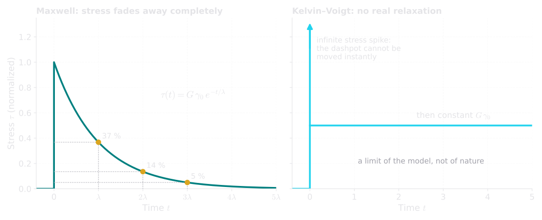
What to look for: the Maxwell model relaxes completely. The Kelvin–Voigt model cannot be stretched instantly at all – a sign that simple models have their limits.

	Maxwell (series)	Kelvin–Voigt (parallel)
Equation	$\dot{\gamma} = \dot{\tau}/G + \tau/\eta$	$\tau = G\gamma + \eta\dot{\gamma}$
Characteristic time	relaxation time $\lambda = \eta/G$	retardation time $\lambda_{ret} = \eta/G$
Under constant load	instant jump, then endless flow	slow approach to a final value
After unloading	partial recovery, permanent deformation	complete but delayed recovery
Under constant deformation	stress relaxes to zero	stress stays (after an infinite spike)
Type of material	viscoelastic liquid	viscoelastic solid
Everyday example	Silly Putty	memory foam

Common pitfall – two elements are not enough: The Maxwell and Kelvin–Voigt models are thinking tools. Real materials show both an instant elastic response and delayed elasticity and flow, and they have not one but many relaxation times. In Part 5 we combine the two models into the four-element Burgers model; in Part 6 we use whole families of Maxwell elements – a “relaxation spectrum”.

When Elastic Liquids Flow: Normal Stresses

So far we have only looked at stresses acting along the direction of shear. Viscoelastic liquids have a remarkable additional property: when they flow, they also push and pull perpendicular to the flow direction. These forces are called normal stresses.

The reason lies in their long molecules. At rest, polymer chains are coiled up like balls of wool. In a flow, they are stretched and aligned along the streamlines – and like stretched rubber bands, they want to contract again. When the streamlines are curved, for example around a rotating stirrer, these “rubber bands” wrap around the stirrer and squeeze the liquid inward.

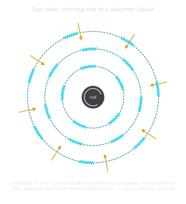
What to look for: the stretched chains pull along the circles like tightened belts. The result is a pressure toward the center – the liquid has to escape somewhere, and the only way out is up.

Physicists describe these effects with two normal stress differences. With direction 1 as the flow direction, direction 2 perpendicular to the sheared layers and direction 3 as the neutral (sideways) direction:

$N_1 = \sigma_{11} - \sigma_{22}, \qquad N_2 = \sigma_{22} - \sigma_{33}$

In words: $N_1$, the first normal stress difference, measures how much more the liquid pulls along the flow direction than perpendicular to the layers – the “rubber band tension” along the streamlines. $N_2$ is usually much smaller and negative, about −10 to −30 % of $N_1$. For Newtonian liquids like water or honey, both are zero. Both are measured in pascal.

At low shear rates, $N_1$ grows with the square of the shear rate, while the shear stress grows only linearly:

$N_1 = \Psi_1\,\dot{\gamma}^2, \qquad \tau = \eta\,\dot{\gamma}$

In words: $\Psi_1$ (“psi one”) is the first normal stress coefficient. Because of the square, normal stresses are negligible in slow flows but become dominant in fast ones.

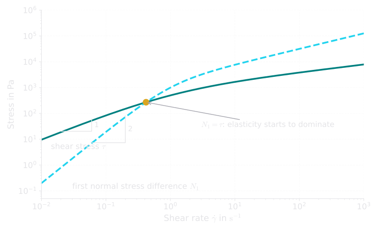
What to look for: the dashed line rises twice as steeply. Beyond the goldenrod crossover, the “rubber band” forces are larger than the shear stress itself (model data).

In the lab – measuring normal forces: In a cone-plate geometry, the first normal stress difference pushes the cone upward. The rheometer’s normal force sensor measures this force $F_N$, and $N_1 = 2F_N / (\pi R^2)$. Example: a cone with radius $R = 25$ mm and a normal force of 1 N gives $N_1 \approx 1$ kPa. Before the measurement, the normal force must be zeroed and the sample must have relaxed from loading.

Rod Climbing: The Weissenberg Effect

The most spectacular consequence of normal stresses was described by Karl Weissenberg in 1947. When a rod rotates in water, the water is flung outward and forms a dip around the rod. When the same rod rotates in a polymer solution or a dough, the liquid climbs up the rod.

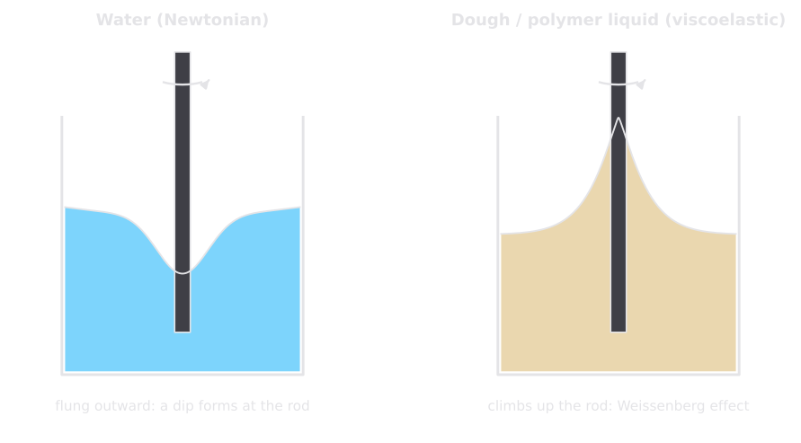
What to look for: the same stirring, opposite surface shapes. In the viscoelastic liquid, the inward squeeze of the stretched chains is stronger than the centrifugal force.

Try it at home – climbing dough: Watch a stand mixer kneading a bread dough with a dough hook. Instead of being flung against the wall of the bowl, the dough winds its way up the hook – sometimes all the way to the top. That is the Weissenberg effect in your kitchen.

Die Swell: When the Extrudate Gets Thicker

A second well-known effect appears when a polymer melt is pressed through a nozzle (a “die”), for example in plastic extrusion or pasta production. The strand that leaves the nozzle is thicker than the nozzle opening.

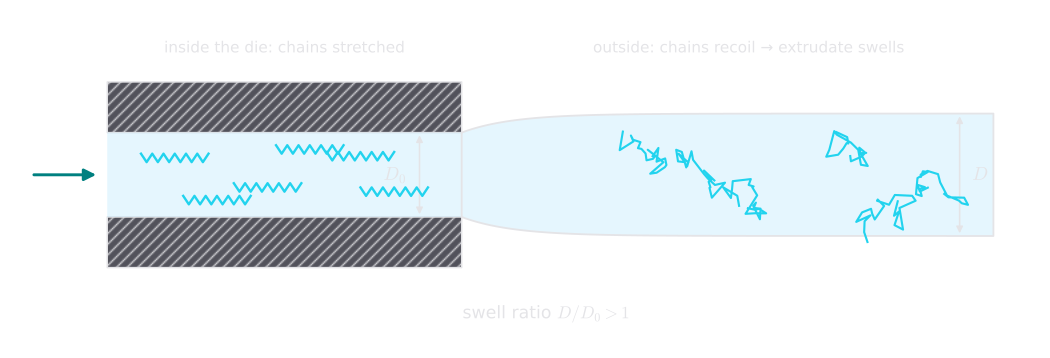
What to look for: inside the die, the chains are stretched; outside, they are free to recoil – they “remember” their coiled shape, and the strand swells.

The swell ratio $D/D_0$ depends on how strongly the chains were stretched, which is described by the ratio of the normal stress difference to the shear stress at the wall $\tau_w$. A classic estimate by Roger Tanner reads

$\frac{D}{D_0} = 0.1 + \left[1 + \frac{1}{2}\left(\frac{N_1}{2\,\tau_w}\right)^2\right]^{1/6}$

In words: the larger the normal stress compared with the shear stress, the more the extrudate swells. The constant 0.1 accounts for the small swell that even a Newtonian liquid shows.

Worked example. If $N_1$ is twice the wall shear stress ($N_1/(2\tau_w) = 1$), the formula gives $D/D_0 = 0.1 + 1.5^{1/6} \approx 1.17$ – the strand is 17 % thicker than the nozzle. Die designers compensate for this by making the nozzle correspondingly smaller.

Why It Matters for Adhesives

A pressure-sensitive adhesive is the Silly Putty principle turned into a product. When you press a tape onto a surface, the contact lasts seconds: the Deborah number is small, and the adhesive behaves like a liquid – it flows into the tiny roughness of the surface and makes intimate contact. When you peel the tape off, the deformation happens within milliseconds: the Deborah number is large, and the adhesive behaves like a tough, solid-like material that resists being pulled away.

This dual character – liquid when bonding, solid when debonding – is exactly what the Chang Viscoelastic Window captures in Part 8, by looking at the adhesive at a slow and a fast time scale. And the stretched, recoiling polymer chains that make dough climb up a hook are the same ones that form the long threads (fibrils) you can see when you slowly peel a label from a bottle.

Key Takeaways

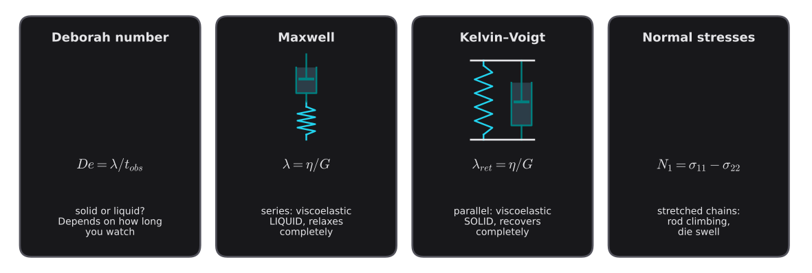
• Viscoelastic materials both store energy (spring) and dissipate it (dashpot). Which behavior dominates depends on the time scale.
• The Deborah number $De = \lambda/t_{obs}$ tells whether a material appears solid ($De \gg 1$) or liquid ($De \ll 1$) – even mountains flow if you wait long enough.
• The Maxwell model (series) describes a viscoelastic liquid: its stress relaxes completely, and under a constant load it flows without limit.
• The Kelvin–Voigt model (parallel) describes a viscoelastic solid: it deforms and recovers with a delay, but always completely.
• The characteristic time $\lambda = \eta/G$ is the material’s “memory time” – after one $\lambda$, 37 % of a relaxing stress remains.
• In flowing polymer liquids, stretched chains create normal stresses ($N_1 > 0$) that grow with the square of the shear rate – visible as rod climbing and die swell.

Key Terms

Term	Meaning in plain language	Symbol, unit
Viscoelastic	Partly elastic (storing), partly viscous (flowing)	–
Relaxation time	The material’s “memory time”	$\lambda$, s
Retardation time	How long a delayed elastic deformation takes	$\lambda_{ret}$, s
Deborah number	Material time divided by observation time	$De$, –
Maxwell model	Spring and dashpot in series – viscoelastic liquid	–
Kelvin–Voigt model	Spring and dashpot in parallel – viscoelastic solid	–
Stress relaxation	Fading of stress at constant deformation	–
Normal stress difference	Push or pull perpendicular to the shear direction	$N_1$, $N_2$, Pa
First normal stress coefficient	Links $N_1$ to the square of the shear rate	$\Psi_1$, Pa·s²
Weissenberg effect	A viscoelastic liquid climbing up a rotating rod	–
Die swell	Extrudate becoming thicker than the die	$D/D_0$, –

Coming Up Next

You tape a poster to the wall in the evening – and in the morning it has slid down a few centimeters. Nobody pulled it; its own weight did the work all night. In Part 5 we look at this slow deformation under constant load, called creep, learn how it is measured with a rheometer, and see what it reveals about the holding power of adhesive tapes.

References

1. Mezger, T. G.: The Rheology Handbook, 5th ed., Vincentz Network, Hanover 2020.
2. Macosko, C. W.: Rheology: Principles, Measurements, and Applications, Wiley-VCH, New York 1994.
3. Morrison, F. A.: Understanding Rheology, Oxford University Press, New York 2001.
4. Reiner, M.: The Deborah Number, Physics Today 17 (1964) 62.
5. Weissenberg, K.: A continuum theory of rheological phenomena, Nature 159 (1947) 310–311.
6. Tanner, R. I.: A theory of die-swell, Journal of Polymer Science Part A-2 8 (1970) 2067–2078.