1 Why a 0.1 % Crosslinker Breaks Your Mixture Design

Picture a typical lab task. You want to tune a waterborne pressure-sensitive adhesive made from three ingredients:

• an acrylic PSA dispersion (the base polymer),
• a tackifier dispersion, for example a rosin ester,
• a crosslinker at around 0.1 %.

The DoE software offers a “mixture design”, because the three ingredients add up to 100 %. So all three go in as mixture components, the runs are made, peel and shear are measured, and the model comes back. The crosslinker coefficient for peel reads −6,400 N/25 mm. The standard errors are enormous, and some effects point in directions that contradict everything you know about the chemistry.

Nothing is wrong with the software, and nothing is wrong with your lab work. The problem is the set-up. This article explains four reasons why a trace component does not belong in a classical mixture model, and shows a simple design that answers the same question cleanly.

The Example Recipe

All numbers in this article come from one consistent, illustrative example. The responses are invented but chemically plausible; the statistical quantities are calculated.

Component	Role	Range (dry, wt% of total solids)
Acrylic PSA dispersion (55 % solids)	base polymer	balance: 69.85–89.95 %
Tackifier dispersion (55 % solids)	raises $T_g$, dilutes the modulus	10–30 %
Crosslinker (e.g. polyaziridine)	links carboxyl groups of the polymer	0.05–0.15 %

Lesson 0: work on a dry basis. Water evaporates; it is not a component of the adhesive film. If you define the recipe on a wet basis, every batch-to-batch variation in solids content (easily ±1 %) adds noise to every factor.

The software builds a 3×3 grid of blends and fits the usual Scheffé quadratic model:

$\hat y = \sum_{i=1}^{3}\beta_i x_i + \sum_{i<j}\beta_{ij}\,x_i x_j \qquad\text{with}\qquad x_\mathrm{PSA} + x_\mathrm{T} + x_\mathrm{XL} = 1$

Here $x_i$ are the mass fractions, and the model has no intercept, because the constant is already hidden in the sum $\sum x_i = 1$.

Problem 1: The Coefficient Describes a Blend You Never Made

In a Scheffé model, the linear coefficient $\beta_i$ has a very specific meaning: it is the predicted response of the pure component, i.e. at $x_i = 1$.

For the PSA and the tackifier, that is a mild extrapolation. For the crosslinker it is extreme: you varied it between 0.05 % and 0.15 %, and the coefficient describes a film made of 100 % crosslinker – an extrapolation by a factor of about 1,000.

It is like judging the saltiness of a soup at 100 % salt from tastings at 0.1 %.

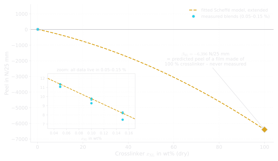
For our example, the fitted peel model delivers:

Coefficient	Value in N/25 mm	Meaning
$\beta_\mathrm{PSA}$	11.3	peel of “pure PSA”
$\beta_\mathrm{T}$	−4.6	peel of “pure tackifier”
$\beta_\mathrm{XL}$	−6,396	peel of “pure crosslinker”
$\beta_\mathrm{PSA \cdot XL}$	4,047	blending term PSA × crosslinker

Huge numbers with opposite signs cancel each other inside the design region. Predictions inside the region can still be fine – the coefficients cannot be interpreted. If you want to know “what the crosslinker does”, read the effect along a direction through the design region (a so-called trace plot along Cox’s direction), never from $\beta_\mathrm{XL}$ itself.

Problem 2: A Razor-Thin Design Region

Now look at the geometry. In the ternary diagram, every possible blend of the three components is a point in the triangle. Our design region spans 20 wt% in the tackifier direction but only 0.1 wt% in the crosslinker direction – a ratio of 200 : 1.

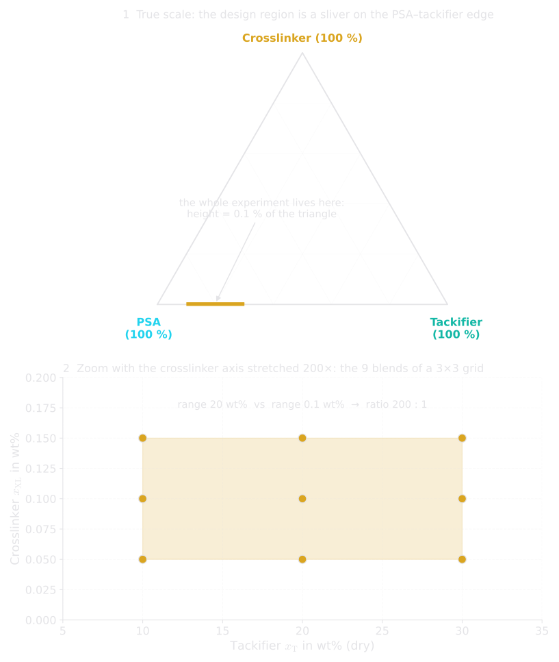
Such a sliver makes the columns of the model matrix almost linearly dependent. The standard measure for this is the condition number

$\kappa = \frac{\sigma_\mathrm{max}(\mathbf X)}{\sigma_\mathrm{min}(\mathbf X)}$

the ratio of the largest to the smallest singular value of the model matrix $\mathbf X$. An orthogonal factorial design has $\kappa = 1$; a common rule of thumb is to stay below about 10 for response-surface designs. A large $\kappa$ means that tiny errors in the data are amplified into large errors in the coefficients.

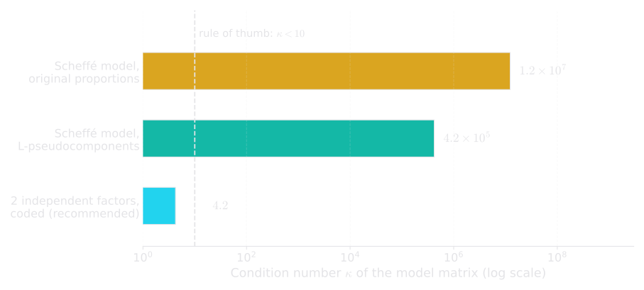
Model on the same 9 blends	$\kappa$	Std. error of the crosslinker coefficient
Scheffé, original proportions	$1.2 \times 10^{7}$	$2.8 \times 10^{6}\,\sigma$
Scheffé, L-pseudocomponents	$4.2 \times 10^{5}$	$1.1 \times 10^{5}\,\sigma$
Two independent factors, coded	4.2	$0.41\,\sigma$

With a realistic test scatter of $\sigma = 0.3$ N/25 mm for peel, the standard error of $\beta_\mathrm{XL}$ in the first row is about 850,000 N/25 mm. No significance test can survive that.

Why pseudocomponents do not rescue this case

The textbook remedy for constrained mixtures are L-pseudocomponents:

$X_i = \frac{x_i - L_i}{1 - \sum_k L_k}$

where $L_i$ are the lower bounds. They re-scale the region so that it starts at zero – but they divide all components by the same total free range, here $1 - \sum L_k = 0.201$. That range is dominated by the tackifier. The crosslinker pseudocomponent then only runs from 0 to 0.005, so the sliver stays a sliver. The condition number improves by a factor of 30, yet stays more than 40,000 times above the rule of thumb.

Problem 3: The Crosslinker Reacts With the Polymer, Not With “the Total”

This is the chemist’s argument, and it is the most important one. A crosslinker consumes the functional groups of the polymer, for example carboxyl groups. What controls the network is therefore the amount of crosslinker per polymer, expressed in phr (parts per hundred parts of polymer):

$c_\mathrm{XL}\,[\mathrm{phr}] = 100\,\frac{x_\mathrm{XL}}{x_\mathrm{PSA}}$

In a mixture design, however, the crosslinker is fixed as a share of the total. When the tackifier goes up, the polymer share goes down – and every chain gets more crosslinks, although the recipe still says “0.1 %”.

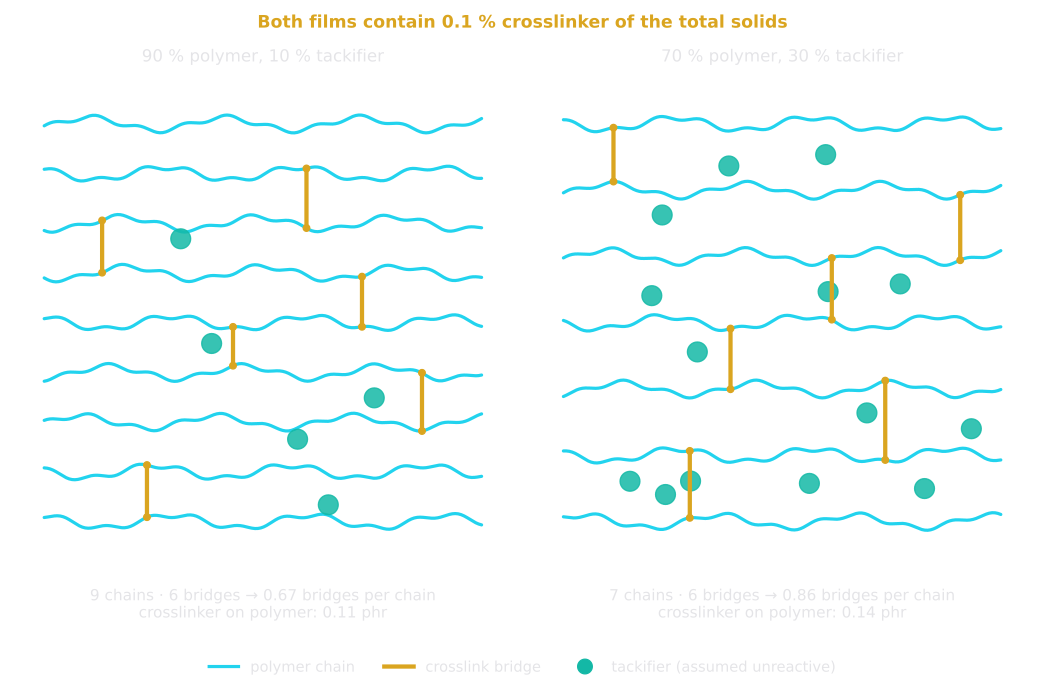
The numbers make it concrete. At a fixed 0.15 % crosslinker of the total, raising the tackifier from 10 % to 30 % raises the crosslinker on polymer from 0.167 to 0.215 phr – plus 29 %.

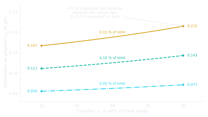
The consequence: what the mixture model reports as a “tackifier effect” is partly a hidden crosslinker effect. The two factors are confounded. Since crosslink density drives shear, peel and tack very strongly, this is not a small bias.

There can be a second layer: acid-functional tackifiers such as some rosin types may also react with certain crosslinkers. If that applies to your system (ask your supplier), the tackifier–crosslinker interaction becomes even harder to read.

Problem 4: Lab Reality

Even a perfect model cannot fix what happens at the bench.

Dosing precision

0.10 % of a batch with 110 g of solids is 0.11 g of active crosslinker. On a balance with 0.01 g readability, rounding alone means ±0.005 g – that is ±4.5 % of the dose, before any losses on the pipette or the beaker wall. Pre-diluting the crosslinker to 10 % active raises the weighed mass to 1.10 g and shrinks the rounding error to ±0.45 %.

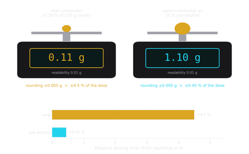
A common worry is that the weighing error of the main components “drowns” the crosslinker signal. It does not: a ±0.3 % error on the PSA dispersion shifts the PSA/tackifier ratio only marginally. The crosslinker acts through its chemistry, not through the 0.1 % it displaces. The relevant noise is the relative dosing error of the crosslinker itself.

Pot life, curing, noise

• Pot life and time to coating. Many waterborne crosslinkers keep reacting or slowly hydrolyse in the wet dispersion. The time between mixing and coating becomes a hidden factor – fix it, or at least record it and randomize the run order.
• Drying and curing. Temperature and time are process factors. They are not components and do not belong into the 100 % sum.
• Response noise. Static shear (holding power) scatters strongly and often spans decades. Model $\log_{10}$ of the shear time and plan replicates.

The Fix: Two Independent Factors Instead of Three Components

Here is the key insight. With only two main components, the mixture part of the problem has just one degree of freedom: the PSA/tackifier ratio. The crosslinker is not a building block of the film; it is a reactive additive. So treat it as what it is:

• Factor 1: tackifier level, in wt% of the PSA + tackifier base (10–30 %) or in phr on polymer.
• Factor 2: crosslinker in phr on polymer solids (e.g. 0.05–0.20 phr).

Both factors can now be varied independently. The problem becomes a plain two-factor response-surface study with the familiar model

$\hat y = b_0 + b_1 z_1 + b_2 z_2 + b_{12}\,z_1 z_2 + b_{11}\,z_1^2 + b_{22}\,z_2^2$

where $z_1$ and $z_2$ are the factors coded from −1 to +1. The condition number drops to about 4, and every coefficient has a direct meaning: $b_2$ is “more crosslinker per polymer”, $b_{12}$ tells you whether the crosslinker acts differently at high tackifier content.

Run it in two stages

1. Stage 1: a classical 2² factorial (four corners) plus three center points – 7 runs. It estimates both main effects and their interaction; the center points provide the pure error and a check for curvature.
2. Stage 2, if the center points show curvature: add the four face points plus two more center points as a second block – 13 runs in total. Together they form a face-centered central composite design, which supports the full quadratic model.

Crosslinker effects on shear are often strongly non-linear, so plan for stage 2 from the beginning.

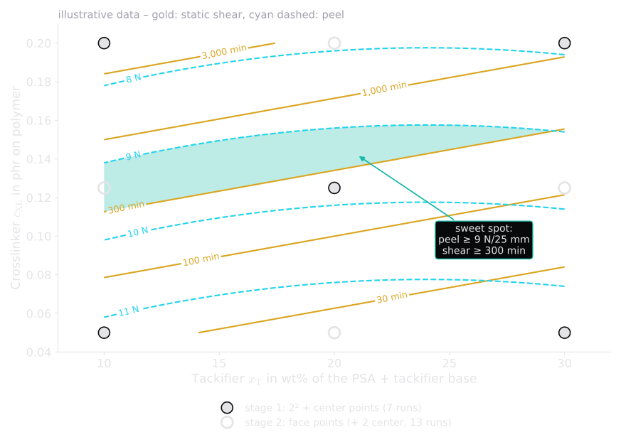
For stage 1, a batch with 100 g of solids looks like this (dispersions at 55 % solids, crosslinker pre-diluted to 10 %):

Run	Tackifier	Crosslinker	PSA dispersion	Tackifier dispersion	Crosslinker solution (10 %)
1	10 %	0.05 phr	163.6 g	18.2 g	0.45 g
2	30 %	0.05 phr	127.3 g	54.5 g	0.35 g
3	10 %	0.20 phr	163.6 g	18.2 g	1.80 g
4	30 %	0.20 phr	127.3 g	54.5 g	1.40 g
5–7	20 %	0.125 phr	145.5 g	36.4 g	1.00 g

Notice runs 2 and 4: less crosslinker solution than in runs 1 and 3, because there is less polymer to react with.

If you must stay with a mixture design

Sometimes the mixture framework is prescribed. Then keep the percentages, but:

• fit a slack-variable model, leaving out the PSA as the “filler” component that makes up the balance, or a Cox model;
• judge component effects with trace plots, never with the raw Scheffé coefficients;
• or treat the crosslinker as a process variable in a combined mixture-process design – which is the same idea as above, expressed in mixture language.

Checklist

1. Define all percentages on a dry basis.
2. Trace components are factors, not mixture components.
3. Dose reactive additives relative to what they react with – phr on polymer.
4. Pre-dilute the crosslinker so that you weigh grams, not centigrams.
5. Check the condition number before running the design (target < 10).
6. Fix the time to coating and curing conditions; model log shear.

Key Takeaways

• A Scheffé coefficient is the response of the pure component. For a 0.1 % ingredient this is an extrapolation by a factor of about 1,000 and cannot be interpreted.
• Very unequal component ranges turn the design region into a sliver; the model becomes ill-conditioned ($\kappa \approx 10^7$), and L-pseudocomponents alone do not cure it.
• Fixing the crosslinker as a share of the total confounds it with the tackifier: +29 % crosslinker per polymer from 10 % to 30 % tackifier.
• The clean route: tackifier level + crosslinker in phr on polymer as two independent factors, run as 2² + center points and extended to a face-centered design if needed ($\kappa \approx 4$).
• In the lab, pre-dilution, dry-basis bookkeeping, fixed pot life and log-transformed shear matter at least as much as the statistics.

Key Terms

• Scheffé model: polynomial for mixtures without intercept; the linear coefficients are the responses of the pure components.
• L-pseudocomponent: re-scaled component that runs from 0 at its lower bound to 1 at its maximum possible share.
• Condition number $\kappa$: ratio of the largest to the smallest singular value of the model matrix; a measure of how strongly data errors are amplified.
• Slack variable: the component left out of the model because it simply makes up the balance to 100 %.
• phr: parts per hundred parts of polymer (resin) solids.
• Confounding: two effects that change together in the design and cannot be separated by the model.

Coming Up Next

Part 2 takes the idea one step further: a formulation with a polymer, two resins and fixed amounts of antioxidant and chalk. Instead of three coupled components, we will use just two ratios – polymer/resin balance and resin split – and see how a classical 2² design turns into a recipe table.

References

• R. H. Myers, D. C. Montgomery, C. M. Anderson-Cook: Response Surface Methodology, 4th ed., Wiley, 2016 – Chapters 12 and 13 (mixture experiments, constrained regions, pseudocomponents, ratios, process variables).
• J. A. Cornell: Experiments with Mixtures, 3rd ed., Wiley, 2002.
• G. E. P. Box, J. S. Hunter, W. G. Hunter: Statistics for Experimenters, 2nd ed., Wiley, 2005.
• R. B. Crosier: “Mixture Experiments: Geometry and Pseudo-Components”, Technometrics 26 (1984) 209–216.
• D. C. Montgomery, S. R. Voth: “Multicollinearity and Leverage in Mixture Experiments”, Journal of Quality Technology 26 (1994) 96–108.
• G. F. Piepel, J. A. Cornell: “Mixture Experiment Approaches: Examples, Discussion, and Recommendations”, Journal of Quality Technology 26 (1994) 177–196.