2 Two Ratios Instead of Three Components: Designing a Polymer–Resin Blend

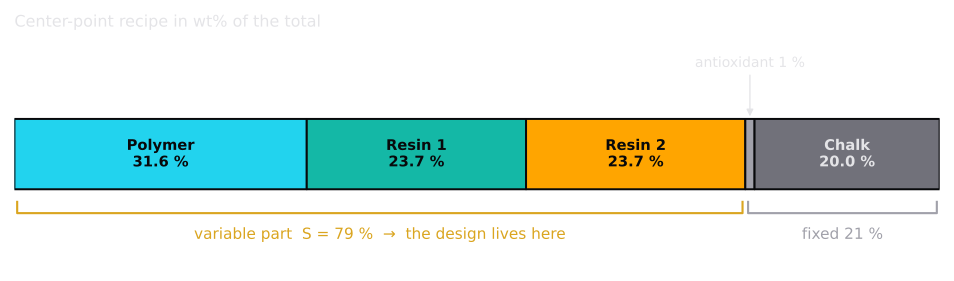
Here is a typical recipe card for a solvent-free pressure-sensitive adhesive:

• a polymer, for example a styrenic block copolymer or an acrylic,
• resin 1, for example an aliphatic resin that is compatible with the soft phase of the polymer,
• resin 2, for example a partly aromatic, modifying resin,
• 1 % antioxidant and 20 % chalk as filler – both fixed.

The task: find the best combination of polymer, resin 1 and resin 2. Strictly speaking this is a mixture problem, because the three ingredients share a fixed budget. You could set up a constrained mixture design with extreme vertices and a Scheffé model.

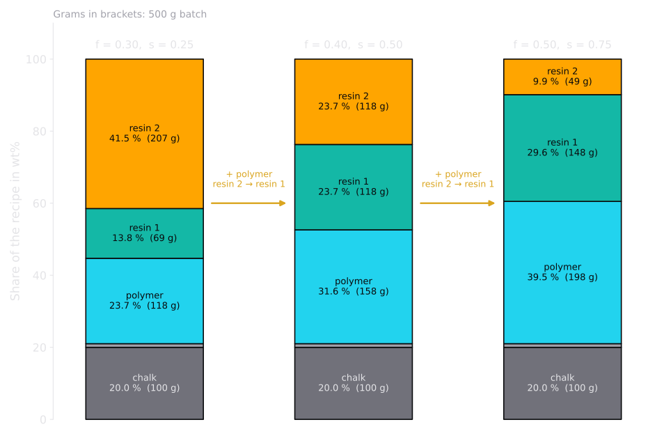
But listen to how formulators actually talk. Nobody says “23.7 % polymer, 13.8 % resin 1, 41.5 % resin 2”. They say “how much resin per polymer?” and “which resin mix?”. This article shows that the experiment can be designed exactly in those two terms – with a classic 2² factorial as the starting point.

In Part 1 we saw what goes wrong when a 0.1 % crosslinker is squeezed into a mixture model. The cure there was to replace coupled components by independent factors. Here we apply the same idea to the main ingredients.

Step 1: Separate the Fixed Part

Antioxidant and chalk do not change, so they take a constant share out of the recipe. What is left is the variable part:

$S = 1 - x_\mathrm{AO} - x_\mathrm{chalk} = 1 - 0.01 - 0.20 = 0.79$

All design decisions happen inside these 79 %.

What does “fixed” really mean?

This is the lesson from Part 1 in a new disguise. If the antioxidant is fixed at 1 % of the total, the amount per polymer changes with the recipe:

Polymer share of the variable part	Antioxidant on polymer
30 %	4.2 phr
40 %	3.2 phr
50 %	2.5 phr

If the antioxidant is there to protect the polymer, it is more consistent to fix it in phr on polymer instead. The same applies to anything that “belongs” to one component.

Chalk fixed in wt% is fine for the design. Keep in mind that stiffness and flow follow the volume fraction of the filler; as long as its mass share is constant and the densities of polymer and resins are similar, the volume fraction stays practically constant too.

Step 2: Two Ratio Factors Instead of Three Components

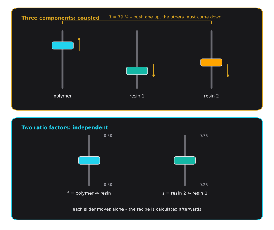
Now replace the three coupled components by two numbers that anybody in the lab understands:

$f = \frac{x_P}{x_P + x_{R1} + x_{R2}} \qquad\qquad s = \frac{x_{R1}}{x_{R1} + x_{R2}}$

• $f$ is the polymer share of the variable part – the polymer/resin balance.
• $s$ is the resin split – the share of resin 1 in the total resin.

The decisive property: $f$ and $s$ are independent. You can move one without touching the other, exactly like the two sliders on a mixing desk. With three components, every move of one slider forces the others to follow.

Every pair $(f, s)$ translates back into exactly one recipe:

$x_P = S\,f,\qquad x_{R1} = S\,(1-f)\,s,\qquad x_{R2} = S\,(1-f)\,(1-s)$

A classic alternative is the ratio $R = x_P/(x_{R1}+x_{R2})$, which equals $f/(1-f)$. Both work. The shares $f$ and $s$ are bounded between 0 and 1 and are easy to code; if you prefer $R$ and it spans a wide range, use $\log R$ as the factor.

In the statistical literature this approach is known as mixture experiments with ratio variables. Because the ratios are independent, any standard response-surface design can be used on them.

Step 3: Start Small – a 2² Design With Center Points

For our example we choose the ranges from experience:

Factor	Low (−1)	Center (0)	High (+1)
Polymer share $f$	0.30	0.40	0.50
Resin split $s$	0.25	0.50	0.75

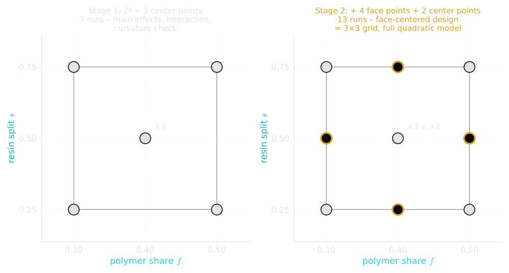
Stage 1 is a classic 2² factorial – the four corners – plus three replicates in the center: 7 runs. It supports the model

$\hat y = b_0 + b_1 z_f + b_2 z_s + b_{12}\,z_f z_s$

with the coded factors $z_f$ and $z_s$ running from −1 to +1. The design is orthogonal (condition number 1.3), so every effect is estimated independently.

The three center points do two jobs. They give an estimate of the pure error, and they allow a curvature check: if the surface were flat, the mean of the center points would equal the mean of the corners. The size of the gap is tested with

$SS_\mathrm{curv} = \frac{n_F\,n_C\,(\bar y_F - \bar y_C)^2}{n_F + n_C}$

with $n_F = 4$ corner runs and $n_C = 3$ center runs (one degree of freedom).

In our illustrative example, peel gives these results:

Run	$f$	$s$	Peel in N/25 mm
1	0.30	0.25	8.91
2	0.50	0.25	9.51
3	0.30	0.75	9.87
4	0.50	0.75	11.55
5–7	0.40	0.50	11.91 / 11.84 / 12.17

The corners average 9.96 N/25 mm, the center points 11.97 N/25 mm. A flat surface cannot explain a gap of 2.0 N/25 mm: the curvature test gives $F \approx 230$, far above the critical value of 18.5 for 1 and 2 degrees of freedom.

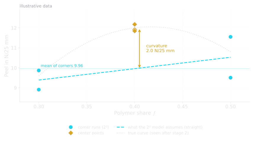
This is typical: peel against resin content usually passes through a maximum. One limitation must be clear, though. The curvature test tells you that the surface is curved, not whether $f$ or $s$ is responsible. That needs stage 2.

Step 4: Augment When the Surface Is Curved

Stage 2 adds the four face points – each factor at its middle level on the edges of the square – plus two more center points: 6 more runs, 13 in total. Together with stage 1 this forms a face-centered central composite design. For two factors its points are exactly the 3×3 grid, and the full quadratic model can now be fitted.

Two practical details:

• Run stage 2 as a second block and include a block term in the model. If a new resin batch or a different room climate shifts all results a little, the block term absorbs it instead of the factor effects.
• Nothing from stage 1 is wasted – the seven runs become part of the final design. This is sequential experimentation: small investment first, extend only where the data ask for it.

From factors back to recipes

Before you run anything, translate every point back into a recipe and check it against the limits of the individual components:

Stage	$f$	$s$	Polymer	Resin 1	Resin 2	Resin/polymer
1	0.30	0.25	23.70	13.82	41.47	2.33
2	0.30	0.50	23.70	27.65	27.65	2.33
1	0.30	0.75	23.70	41.47	13.82	2.33
2	0.40	0.25	31.60	11.85	35.55	1.50
1 + 2	0.40	0.50	31.60	23.70	23.70	1.50
2	0.40	0.75	31.60	35.55	11.85	1.50
1	0.50	0.25	39.50	9.88	29.62	1.00
2	0.50	0.50	39.50	19.75	19.75	1.00
1	0.50	0.75	39.50	29.62	9.88	1.00

All values in wt% of the total; every run also contains 1.0 % antioxidant and 20.0 % chalk.

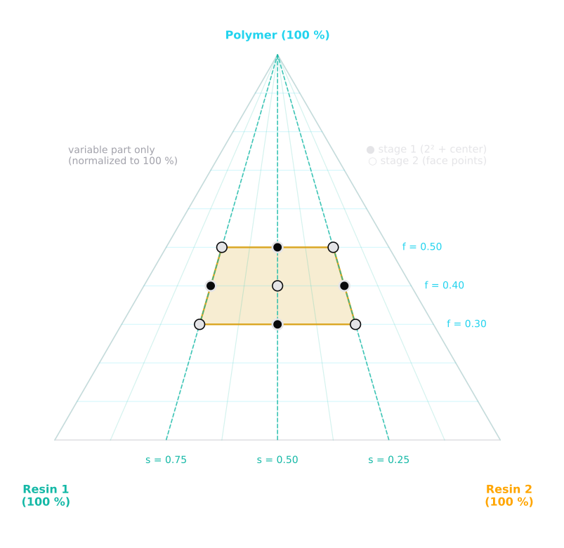
In the ternary diagram of the variable part, the square in $(f, s)$ becomes a trapezoid. Lines of constant resin split are rays from the polymer corner; lines of constant polymer share run parallel to the resin 1–resin 2 edge.

Step 5: Model and Interpretation

After stage 2, the full quadratic model for peel reads (coded factors, block term omitted):

$\hat y_\mathrm{peel} = 12.08 + 0.62\,z_f + 0.94\,z_s + 0.27\,z_f z_s - 1.66\,z_f^2 - 0.41\,z_s^2$

The standard errors are 0.13 for the linear terms and 0.19 for the quadratic terms. The block term is small (0.08) – no relevant shift between the two stages. The condition number of the whole design including the block is 3.2.

This is where the ratio factors pay off. Every coefficient has a formulator’s meaning:

• $b_1 = 0.62$: more polymer, less resin → peel rises slightly …
• $b_{11} = -1.66$: … but strongly curved – there is an optimum polymer share inside the range.
• $b_2 = 0.94$: replacing resin 2 by resin 1 raises peel.
• $b_{12} = 0.27$: the benefit of resin 1 is somewhat larger at high polymer share – a small interaction.

For static shear (modelled as $\log_{10}$ of the holding time), the picture is simpler: more polymer increases shear clearly, more resin 1 lowers it slightly.

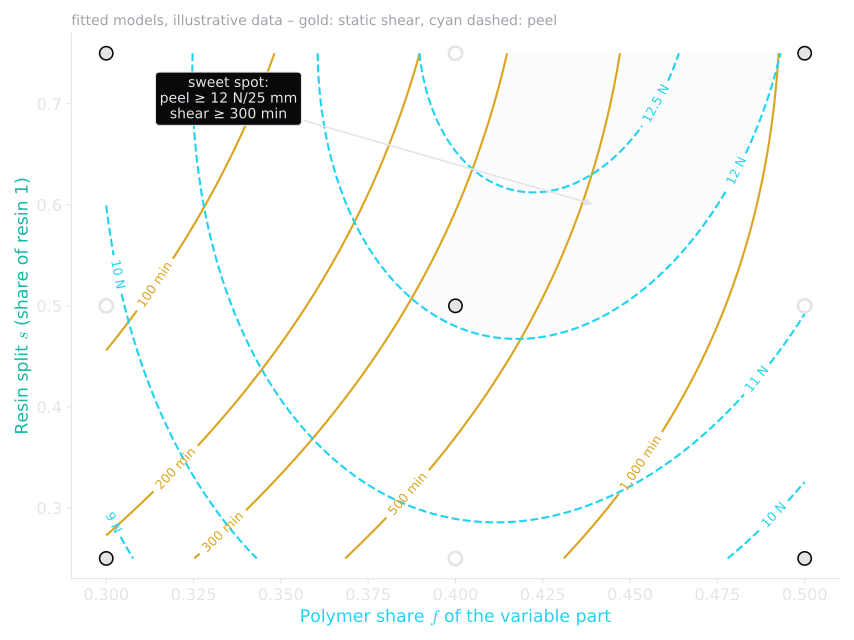
Peel reaches its maximum of about 12.7 N/25 mm at $f \approx 0.43$ and $s = 0.75$, with a static shear of about 360 min. As a recipe: 33.7 % polymer, 34.0 % resin 1, 11.3 % resin 2, plus 1 % antioxidant and 20 % chalk. The optimum sits on the edge of the range ($s = 0.75$) – a clear hint to extend the resin split in a follow-up experiment.

Why does the surface look like this? The polymer share mainly shifts the glass transition temperature and dilutes the plateau modulus; the resin split changes the compatibility and $T_g$ of the resin phase. How these viscoelastic quantities control tack, peel and shear is explained in the rheology series on the Chang viscoelastic window.

When Ratios Are Not the Best Choice

Ratio factors are convenient, but they have a price:

Aspect	Constrained mixture design (Scheffé)	Ratio factors $(f, s)$
Interpretation	blending coefficients of pure components	“more polymer”, “more resin 1”
Region covered	the whole feasible polytope	a trapezoid inside it
Design	extreme vertices, D- or I-optimal	any standard factorial or response-surface design
Adding process factors	combined mixture-process design, many runs	simply add another factor
Component limits	built into the design	must be checked run by run

Three points deserve attention:

• Coverage. If you need predictions over the entire feasible mixture region, a D- or I-optimal design in the original proportions is the better choice.
• Individual limits. A limit such as “resin 2 at most 35 %” cuts a corner off the ratio square. Always translate back and check every run.
• Model form. A polynomial in ratios is not identical to a Scheffé polynomial. The results are interpreted in terms of the ratios – which is exactly what makes them attractive for formulators.

Step by Step

1. List the fixed components and decide their reference: share of the total or phr on polymer.
2. Compute the variable part $S$.
3. Choose ranges for $f$ and $s$ from experience.
4. Translate all runs – including the later face points – into recipes and check them against component limits.
5. Stage 1: 2² + 3 center points (7 runs); fit main effects and interaction, test for curvature.
6. No curvature → done. Curvature → stage 2: 4 face points + 2 center points as a second block (13 runs in total).
7. Fit the quadratic model in coded factors with a block term; check the condition number and residuals.
8. Report the result as a recipe again.

Key Takeaways

• Remove the fixed components first; the design lives in the variable part $S$. Check whether “fixed” should really mean “fixed per polymer”.
• Three coupled components can be replaced by two independent factors: polymer share $f$ and resin split $s$.
• Start with a 2² design plus center points (7 runs). If the center points reveal curvature, add four face points to reach a face-centered design – nothing from stage 1 is lost.
• Every coefficient then has a direct meaning for the formulator, and the design stays well-conditioned.
• The price: the design covers a trapezoid, not the whole mixture region, and individual component limits must be checked run by run.

Key Terms

• Variable part $S$: share of the recipe that is actually varied, after removing fixed components.
• Ratio variable: a factor defined as a ratio or share of mixture components, such as $f$ and $s$; ratio variables are independent of each other.
• 2² factorial: two factors at two levels each – four runs at the corners of a square.
• Center points: replicated runs in the middle of the design; they estimate pure error and reveal curvature.
• Face-centered central composite design: 2² corners plus face points and center points; for two factors it equals the 3×3 grid.
• Block: a group of runs made under similar conditions, such as one day or one raw-material batch; a block term keeps shifts between groups out of the factor effects.

References

• R. H. Myers, D. C. Montgomery, C. M. Anderson-Cook: Response Surface Methodology, 4th ed., Wiley, 2016 – Chapter 13 (constrained mixtures, ratios of components, process variables).
• J. A. Cornell: Experiments with Mixtures, 3rd ed., Wiley, 2002.
• G. E. P. Box, J. S. Hunter, W. G. Hunter: Statistics for Experimenters, 2nd ed., Wiley, 2005 – factorial designs with center points and sequential experimentation.
• G. F. Piepel, J. A. Cornell: “Mixture Experiment Approaches: Examples, Discussion, and Recommendations”, Journal of Quality Technology 26 (1994) 177–196.
• S. M. Kowalski, J. A. Cornell, G. G. Vining: “Split-Plot Designs and Estimation Methods for Mixture Experiments with Process Variables”, Technometrics 44 (2002) 72–79.